5  Computing Homology

Sequence comparison algorithms are a key piece in the family of tools used in bioinformatics. These algorithms look for protein or DNA sequences that resemble a sample sequence you already know. This laboratory introduces the BLAST set of tools and multiple alignment.

By the end of this laboratory you will be able to:

• explain sequence homology, orthology/paralogy, and how e-values quantify similarity
• choose the right BLAST flavour (blastp, tblastn, blastx, tblastx, blastn) for a task
• run protein and DNA similarity searches at NCBI and EBI and interpret the results
• read a BLAST alignment (identities, positives, gaps, masked regions)
• apply homology search to a real problem: characterising the SARS-CoV-2 genome

Significant similarity between two or more sequences suggests they share a common ancestor, similar structure, and biological function. This is surprisingly useful: it can reveal the role of a sequence of unknown function through a similar sequence of known function, possibly even from a different organism.

NoteLab at a glance

Goal: understand sequence homology and run similarity searches and alignments. Prerequisites: Introduction to R; Searching NCBI & Ensembl. Time: ~2.5 h. Packages: Biostrings, pwalign, ape (and rentrez/rBLAST for the optional programmatic search). Deliverable: a lab report.

5.1 Homology

Two sequences are homologous when they share a common ancestor and thus show clear similarities. The concept of homology is central to comparative biology and fundamental to understanding sequence function.

When sequences are homologous, they are also conserved. Conservation refers to a high degree of similarity in protein or orthologous¹ DNA sequences and protein structures. A highly conserved region or protein is usually related to an important function: a mutation in a highly conserved region would likely lead to a non-viable organism, or one strongly disfavoured by natural selection.

From a practical point of view, two sequences can be considered homologous if 25% of amino acids are identical (proteins) or 70% of nucleotides are identical (DNA) — though this holds only for sufficiently long sequences (>100 residues). Homology algorithms report the e-value (the odds that the similarity is due to chance), the length of the similar segments, and the number of insertions/deletions. A reasonable e-value falls below \(10^{-4}\); a useful rule of thumb for interpretation:

• \(E < 10^{-100}\): identical sequence (same gene/protein and organism)
• \(10^{-100} < E < 10^{-50}\): almost identical sequence
• \(10^{-50} < E < 10^{-10}\): closely related sequence
• \(10^{-5} < E < 1\): could be a true homologue
• \(E > 1\): most likely not related

5.2 Alignment types

Over the past decades, computing sequence similarity has improved dramatically. Where similarity was once found by visual inspection, a query is now compared automatically against databases of millions of sequences.

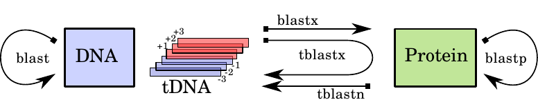
The most famous algorithm in bioinformatics is BLAST — Basic Local Alignment Search Tool. Several flavours target different search types:

1. Nucleotide BLAST — search a nucleotide database with a nucleotide query (blastn, megablast, discontiguous megablast).
2. Protein BLAST — search a protein database with a protein query (blastp, psi-blast, phi-blast).
3. blastx — search a protein database with a translated nucleotide query.
4. tblastn — search a translated nucleotide database with a protein query.
5. tblastx — search a translated nucleotide database with a translated nucleotide query.

These methods are summarised in Figure 5.1.

Figure 5.1: Scheme of the main BLAST search methods.

5.3 Working with protein sequences

This section applies when you have a protein sequence and want to find similar proteins, or DNA that could code for similar proteins. Following Figure 5.1, two methods are available: blastp (protein query against a protein database) and tblastn (protein query against a nucleotide database).

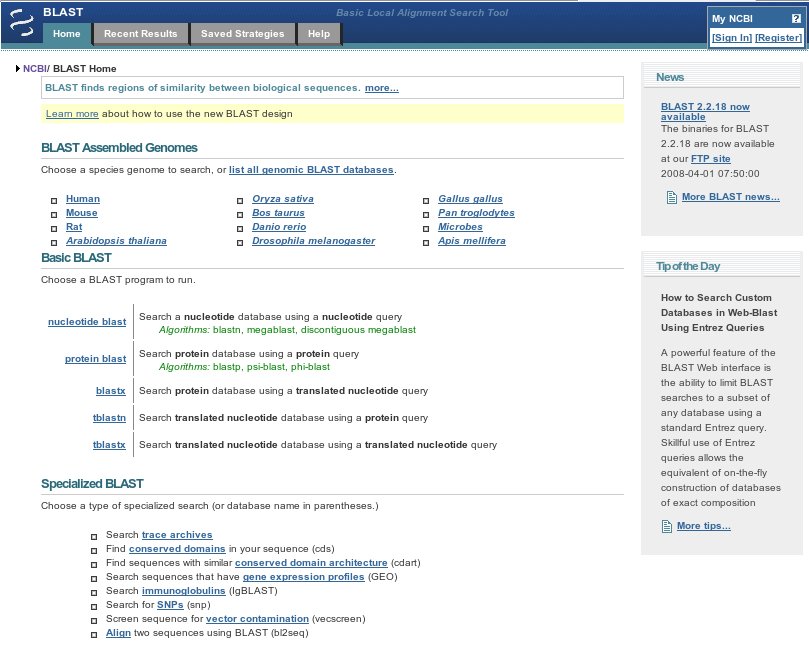
The same BLAST query on different servers can yield different results, because each interface may work with different databases or versions. We use the two main BLAST interfaces (NCBI and EMBnet) and stick to NCBI for the following sections.

Figure 5.2: NCBI BLAST entry site.

5.3.1 BLASTP at NCBI

We will answer whether there are any proteins similar to the human Low-density lipoprotein receptor precursor, found in the SWISS-PROT protein database.

Tip✅ Exercise 5.1 — BLASTP at NCBI

1. Find the BLAST entry point at NCBI (https://blast.ncbi.nlm.nih.gov/).
2. Look for the amino-acid sequence of the LDL receptor (precursor) for Homo sapiens — from the gene search as LDLR.
3. Insert the amino-acid sequence or the accession number into the blastp suite (it accepts a sequence or a SWISS-PROT accession P0XXXX). Run a BLASTP search with default parameters.
4. Which databases did the algorithm cover?
5. Return to the blastp form and select SWISS-PROT in the database selector. List and explain the first 5 hits.
6. Which is the closest protein? What percentage of coincidence do the two share?
7. Open the Distance Tree view and describe the result.

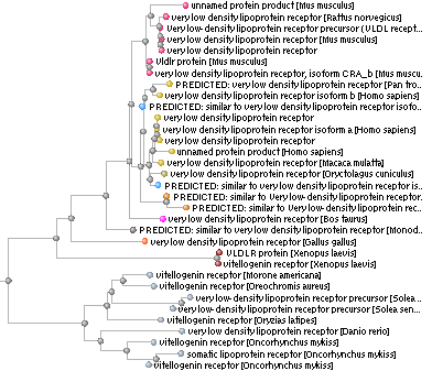Figure 5.3: NCBI BLAST: partial results in tree form.

The graphic display with bars shows which parts of the query sequence match the found protein sequence. Each bar represents a similar region, and its colour indicates match quality — from black (worst) to red (best). Clicking a bar takes you to the corresponding alignment. The hit list below shows the sequence accession, name, and description; each entry links to its database record.

Figure 5.4: NCBI BLAST: alignment section excerpt.

The alignment section (Figure 5.4) shows your query sequence (top) and the found sequence (bottom). In the middle row, an amino-acid letter indicates a match, a + indicates similar residues, and a space indicates a mismatch. The numbers on each side give the residue coordinates of the matching region. Regions marked X usually contain many repeats and are masked by BLAST so they don’t interfere with the search.

Tip✅ Exercise 5.2 — Alignments

1. Why would regions with repeats be masked by BLAST?
2. What are Conserved Domains (CD) in proteins? What is their effect if included in BLAST searches?

TipSolution 5.2

• Low-complexity/repeat regions match non-homologously by chance (they recur everywhere), inflating e-values, so masking them stops spurious hits.
• Conserved domains are evolutionarily conserved functional/structural units of a protein; displaying them (CD-search) flags the biological role of each hit.

5.3.2 TBLASTN at NCBI

Here we seek DNA nucleotide sequences starting from a protein sequence, using tblastn. This takes a protein query and compares it against an NCBI nucleotide database translated in all six reading frames.

Tip✅ Exercise 5.3 — TBLASTN

1. Run a tblastn query with the same protein sequence you used for BLASTP.
2. Comment on the type of the first results and the differences from the BLASTP results.

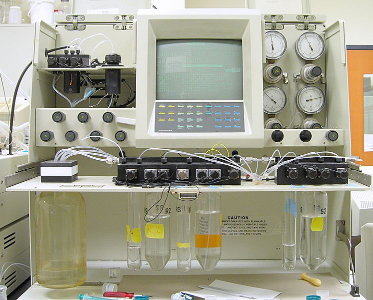Figure 5.5: A Beckman-Coulter Porton LF3000G protein sequencer.

5.3.3 BLASTP at EBI

Protein sequencing determines the amino-acid sequence of a protein, helping to understand its structure and function. Imagine you work in a lab on bio-inspired technologies for computer displays, trying to identify a novel insect protein that would enable organic displays with high electroluminescence at very low power. You suspect you have isolated it — Problem Sequence 1 below.

Tip✅ Exercise 5.4 — BLASTP at EBI

1. Connect to the EBI Sequence Similarity Searching website (https://www.ebi.ac.uk/jdispatcher/sss).
2. Choose PSI-BLAST (Protein Database Query) and paste Problem Sequence 1.
3. Explore the Results sections: Summary, Tool Output, Visual Output, Functional Predictions.
4. Can you hypothesise a function for this protein sequence? Did you find the protein you were looking for?
5. If you find the protein of Sequence 2 in a patient, what would you suggest?
6. If sequences A and B are both homologous to your query C, can you conclude that A is homologous to B?

>sp|Problem Sequence 1
CGGAGKVEYITAPFYPLEDTTAGEQLHKAMKRYALVPGTIAFDAHIEVYQGFQAEYFEMS
VRLAEAMKRYGLNTNHRIVVCSENSLQFFMPVLGALFIGVAVAPANDIYIERELLNSMNI
SQPTVVFVSEEGWQKILNVQKKLPIIQKIIIMDSKTDYQGFQSMYTFVTSHLPPGFNEYD
FVPESFDRDKTIALISNSSGSTGLPKGVALPHRTACVRFSHARDPIFGNQIIPDTAILSV
VPFHHGFGMFTTLGYLICGFRVVLMYRFEEELFLRSLQDYKIQSALLVPTLFSFFAKSTL
IDKYDLSNLHEIASGGAPISKEVGEAVAKRFHLPGIRQGYGLTETTSAILITPEGDDKPG
AVGKVVPFFEAKVVDLDTGKTLGVNQRGELCVRGPMIMSLYVNNPEATNALIDKDGWLHS
AVGKVVPFFEAKVVDLDTGKGLGPKGVALPHRTACVRFSHARDPIFGNQAVAKRFHLPLE
GDIAYWDEDEHFFIVDLLKSLIKYKGYQVAAAALESILLQHPNIFDAGVAGLPDDDAGEL
PAAVVVLEHGKTMTEKEIV

>sp|Problem Sequence 2
MFVFLVLLPLVSSQCVNLTTRTQLPPAYTNSFTRGVYYPDKVFRSSVLHSTQDLFLPFFSNVTWFHAIHV
SGTNGTKRFDNPVLPFNDGVYFASTEKSNIIRGWIFGTTLDSKTQSLLIVNNATNVVIKVCEFQFCNDPF
LGVYYHKNNKSWMESEFRVYSSANNCTFEYVSQPFLMDLEGKQGNFKNLREFVFKNIDGYFKIYSKHTPI
NLVRDLPQGFSALEPLVDLPIGINITRNQFNSAIGRSYLTPGDSSSGWTAGAAAYPIHKELERTFLLKYN
ENGTITDAVDCALDPLSETKCTLKSFTVEKGIYQTSNFRVQPTESIVRFPNITNLCPFGEVFNATRFASV
YAWNRKRISNCVADYSVLYNSASFSTFKCYGVSPTKLNDLCFTNVYADSFVIRGDEVRQIAPGQTGKIAD
YNYKLPDDFTGCVIAWNSNNEEEEEEENYNYLYRLFRKSNLKPFERDISTEIYQAGSTPCNGVEGFNCYF
PLQSYGFQPTNGVGYQPYRVVVLSFELLHAPATVCGPKKSTNLVKNKCVNFNFNGLTGTGVLTESNKKFL
PFQQFGRDIADTTDAVRDPQTLEILDITPCSFGGVSVITPGTNTSNQVAVLYQDVNCTEVPVAIHADQLT
PTWRVYSTGSNVFQTRAGCLIGAEHVNNSYECDIPIGAGICASYQTQTNSPRRARSVASQSIIAYTMSLG
AENSVAYSNNSIAIPTNFTISVTTEILPVSMTKTSVDCTMYICGDSTECSNLLLQYGSFCTQLNRALTGI
AVEQDKNTQEVFAQVKQIYKTPPIKDFGGFNFSQILPDPSKPSKRSFIEDLLFNKVTLADAGFIKQYGDC
LGDIAARDLICSNNSNNSNVLPPLLTDEMIAQYTSALLAGTITSGWTFGAGAALQIPFAMQMAYRFNGIG
VTQNVLYENQKLIANQFNSAIGKIQDSLSSTASASILLQHPNINQNKKLNTLVKQLSSNFGAISSVLNDI
LSRLDKVEAEVQIDRLITGRLQSLQTYVTQQLIRAAEIRASANLAATKMSECVLGQSKRVDFCGKGYHLM
SFPQSAPHGVVFLHVTYVPAQEKNFTTAPAICHDGKAHFPREGVFVSNGTHWFVTQRNFYEPQIITTDNT
FVSGNCDVVIGIVNNTVYDPLQPELDSFKEELDKYFKNHTSPDVDLGDISGINASVVNIQKEIDRLNEVA
KNLNESLIDLQELGKYEQYIKWPWYIWLG

5.4 Working with DNA sequences

Finding similar DNA sequences is harder than finding similar proteins — the amount of data to search through is considerably larger. For DNA queries we have three main tools: blastn, tblastx, and blastx.

5.4.1 BLASTN at NCBI

BLASTN compares a nucleotide query against a nucleotide database. All current BLAST algorithms use BLAST 2.0, which allows gaps in alignments by default, enabling both local and global alignments — suitable for most applications.

5.4.2 BLASTX at NCBI

blastx takes a nucleotide query, translates it in all six frames, and compares those translations to a protein database — useful for finding proteins encoded by a nucleotide query. Because it combines significance statistics across frames, it is especially useful when the reading frame is unknown or the query contains frame-shift errors. It is often the first analysis performed on a newly determined nucleotide sequence and is used extensively for EST analysis; it is more sensitive than nucleotide BLAST because the comparison happens at the protein level.

Tip✅ Exercise 5.5 — BLASTX

1. Find the gene for the human HBG1 hemoglobin, gamma A.
2. Run a blastx with the gene sequence. Compare the results with the gene structure in Figure 5.6.
3. Explain why blastx is more sensitive than nucleotide–nucleotide BLAST.
4. Save the result in a file.

TipSolution 5.5

• blastx returns hits only at the two protein-coding exons of HBG1, matching the structure in Figure 5.6; the intron and UTRs give no protein hit.
• It is more sensitive because it aligns at the protein level: synonymous codons and conservative amino-acid substitutions make distant homologues detectable even when their DNA sequences have diverged.

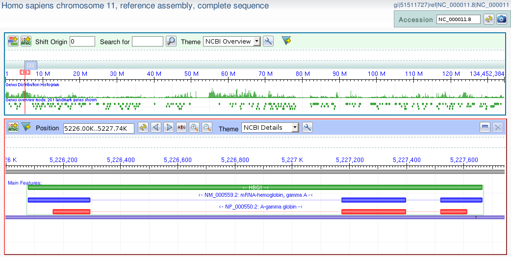Figure 5.6: Structure of the HBG1 hemoglobin, gamma A gene from NCBI.

5.4.3 TBLASTX at NCBI

tblastx takes a nucleotide query, translates it in all six frames, and compares those to database sequences dynamically translated in all six frames — effectively a more sensitive blastp search without manual translation. It circumvents frame-shifts and ambiguities that may hide open reading frames, which is very useful for identifying potential proteins encoded by single-pass EST reads² and for discovering novel genes.

Tip✅ Exercise 5.6 — TBLASTX

1. Run a tblastx with the human HBG1 hemoglobin, gamma A gene sequence. Observe and discuss the results.
2. What is the main difference from the previous methods?
3. Compare the results with the gene structure.

TipSolution 5.6

• blastn: only sequences that are exactly similar at the DNA level (recently diverged). blastx: one fixed protein translation vs the protein DB. tblastx translates both the query and every database entry in all six frames, finding homologous coding regions even between sequences whose DNA has diverged — the most sensitive but slowest of the three.

5.5 SARS-CoV-2

Severe acute respiratory syndrome coronavirus 2 (SARS-CoV-2) is the virus causing COVID-19. The outbreak, which presumably started from a local seafood market, grew to infect 2761 people in China by 26 January 2020 (Zhou et al., 2020). It is the seventh known coronavirus to infect people, after 229E, NL63, OC43, HKU1, MERS-CoV, and the original SARS-CoV (2003).

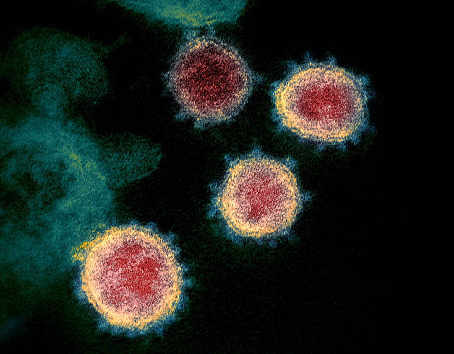Figure 5.7: Transmission electron microscope image of SARS-CoV-2 (from Wikimedia).

The first known SARS-CoV-2 sequence was published on 2 February 2020 (revised 11 February) (Wu et al., 2020) under GenBank annotation MN908947.3, from a single patient — a worker at a local market admitted to the Central Hospital of Wuhan on 26 December 2019 with a severe respiratory syndrome. Metagenomic RNA sequencing of bronchoalveolar lavage fluid identified a new RNA virus of the family Coronaviridae, designated WH-Human 1. Phylogenetic analysis of the complete 29,903-nucleotide genome revealed the virus was most closely related (89.1% nucleotide similarity) to a group of SARS-like coronaviruses (genus Betacoronavirus, subgenus Sarbecovirus) previously found in bats in China.

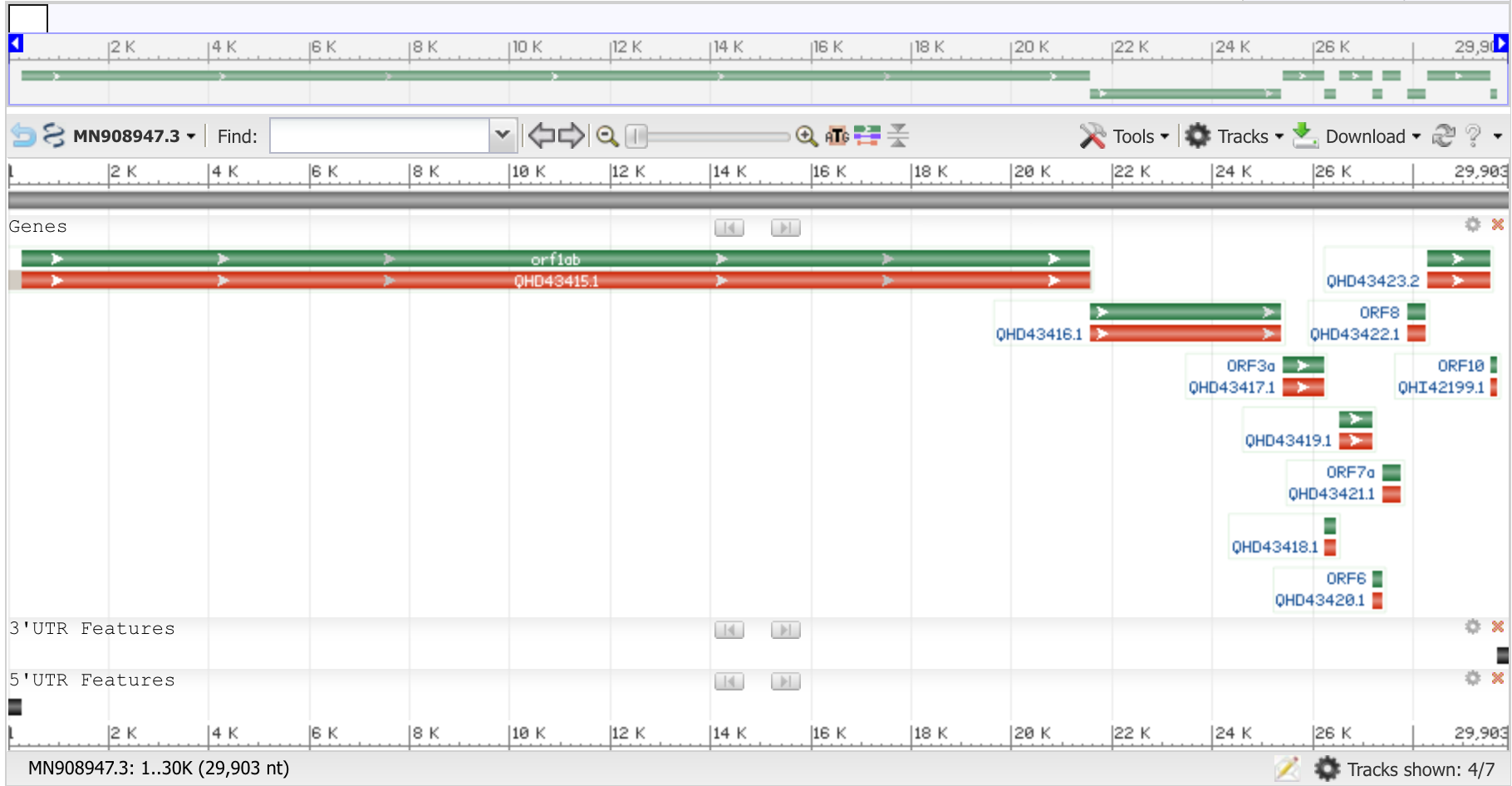Figure 5.8: SARS-CoV-2 isolate Wuhan-Hu-1, complete genome (GenBank MN908947.3).

The genes annotated on MN908947.3 are listed in Table 5.1.

Table 5.1: Genes listed on MN908947.3

#	Accession	Start	Stop	Gene symbol	Strand
1	MN908947.3	266	21555	orf1ab	plus
2	MN908947.3	21563	25384	S	plus
3	MN908947.3	25393	26220	ORF3a	plus
4	MN908947.3	26245	26472	E	plus
5	MN908947.3	26523	27191	M	plus
6	MN908947.3	27202	27387	ORF6	plus
7	MN908947.3	27394	27759	ORF7a	plus
8	MN908947.3	27894	28259	ORF8	plus
9	MN908947.3	28274	29533	N	plus
10	MN908947.3	29558	29674	ORF10	plus

Tip✅ Exercise 5.7 — SARS-CoV-2

1. Run a homology search on the full SARS-CoV-2 sequence. Explain which virus sequences are homologous to 2020 SARS-CoV-2, and in which regions.
2. Plan and run a strategy for analysing the different elements of the SARS-CoV-2 sequence — its proteins and active domains. Learn as much as you can about this virus in terms of homology to any known sequence.

TipSolution 5.7

• A nucleotide blastn of the ~29.9 kb genome returns bat SARS-like coronaviruses (e.g. RaTG13, ~96 % identity) and the 2003 SARS-CoV (~82 %), most conserved in the orf1ab replicase and the nucleocapsid, and most divergent across the S (spike) gene.
• A sensible strategy is to blastn the full genome, blastx each annotated CDS from Table 5.1, and run CD-search on the spike and orf1ab polyprotein to locate the receptor-binding and protease domains.

5.6 Doing it in R

The web interfaces above are how you’ll usually explore a single query, but for reproducible work you want the search and alignment in code. Bioconductor’s Biostrings aligns sequences locally, and ape builds trees — both run offline. We illustrate the mechanics on a small set of synthetic sequences (one seed and progressively more mutated copies), so the results are reproducible anywhere:

library(Biostrings)
library(pwalign)      # pairwiseAlignment()/stringDist() live here since BioC 3.19
set.seed(1)
aa <- strsplit("ACDEFGHIKLMNPQRSTVWY", "")[[1]]
seed <- paste(sample(aa, 80, replace = TRUE), collapse = "")
mutate <- function(s, n) {
  v <- strsplit(s, "")[[1]]; pos <- sample(length(v), n)
  v[pos] <- sample(aa, n, replace = TRUE); paste(v, collapse = "")
}
seqs <- AAStringSet(c(seed = seed, near = mutate(seed, 6),
                      mid = mutate(seed, 18), far = mutate(seed, 34),
                      distant = mutate(seed, 52)))
seqs

AAStringSet object of length 5:
    width seq                                             names               
[1]    80 EHACMQVWALQLHKRFKQFFCL...MTEPISQYHPNSAPGTKHWVSM seed
[2]    80 HHACMQVWANQLHKRFKQFFCL...MREPIMQYHPNSAPGTKHWVSM near
[3]    80 RHACMQVWALQLHKRFKQFFCW...MTCPISQYAPNSAPGTKHWVSM mid
[4]    80 KEKCMQVWLSQIHHLLNQKECL...MTEPIIQFHPRSTPGTEEWGYM far
[5]    80 EWYGMQKGQSDTHFVGSIFTCA...MAPMISWYHPNHRPEMSAGVKM distant

A pairwise alignment with BLOSUM62 scores similarity — high for the near copy, low for the distant one, exactly as an e-value would rank them:

pa_near <- pairwiseAlignment(seqs[["seed"]], seqs[["near"]],
                             substitutionMatrix = "BLOSUM62",
                             gapOpening = 10, gapExtension = 4)
pa_far  <- pairwiseAlignment(seqs[["seed"]], seqs[["distant"]],
                             substitutionMatrix = "BLOSUM62",
                             gapOpening = 10, gapExtension = 4)
c(near = score(pa_near), distant = score(pa_far))

   near distant 
    428     112 

pid(pa_near)   # percent identity of the close pair

[1] 92.5

From all-vs-all distances we can build and draw a neighbour-joining tree (Figure 5.9), the same idea as the BLAST “Distance Tree view”:

library(ape)
d <- stringDist(seqs, method = "hamming")
plot(nj(d), type = "unrooted", cex = 0.9, no.margin = TRUE)

Figure 5.9: Neighbour-joining tree of the illustrative sequences, recovering the mutation order from the seed.

NoteSearching a real database from R

To search NCBI itself, fetch sequences with rentrez and run BLAST locally with rBLAST (a wrapper around NCBI BLAST+). These need network access and a BLAST install, so they are shown, not run here:

library(rentrez); library(rBLAST)
ldlr <- entrez_fetch(db = "protein", id = "NP_000518", rettype = "fasta")
# ... write to a FASTA, then:  blast(db = "swissprot") |> predict(query)

For multiple alignment and publication-quality trees, add msa/DECIPHER and ggtree.

5.7 Further reading

• Altschul et al. (1990), J. Mol. Biol. — the original BLAST paper.
• NCBI BLAST documentation and the EBI Job Dispatcher help.
• The Biostrings / pwalign and ape vignettes for the in-R alignment and tree code.

Worked solutions for the exercises are in the collapsed callouts below each exercise.

5.8 Report

Write a laboratory report following the structure of this text. It should contain an introduction, the goals of each section, and a description of the results of each part. Include any graphics relevant to making your work understandable. The lab should be delivered within two weeks.

Wu, F., Zhao, S., Yu, B., Chen, Y.-M., Wang, W., Song, Z.-G., Hu, Y., Tao, Z.-W., Tian, J.-H., Pei, Y.-Y., et al. (2020). A new coronavirus associated with human respiratory disease in china. Nature, 579(7798), 265–269.

Zhou, P., Yang, X.-L., Wang, X.-G., Hu, B., Zhang, L., Zhang, W., Si, H.-R., Zhu, Y., Li, B., Huang, C.-L., et al. (2020). A pneumonia outbreak associated with a new coronavirus of probable bat origin. Nature, 1–4.

---

1. Homologous sequences are orthologous if they were separated by a speciation event: when a species diverges into two, the divergent copies of a single gene are orthologous. They are paralogous if separated by a gene duplication event: if a gene is duplicated to occupy two positions in the same genome, the two copies are paralogous.

2. An expressed sequence tag (EST) is a short sub-sequence of a transcribed, spliced nucleotide sequence (coding or not).