Code
library(gaston)
geno  <- read.bed.matrix("data/ge03d2")
Reading data/ge03d2.rds
Reading data/ge03d2.bed Code
pheno <- read.table("data/ge03d2.phe", header = TRUE)In this lab we explore the steps taken in a genome-wide association (GWA) analysis: exploring a dataset, running a first association scan, discovering that it is confounded, cleaning the data, and re-running the scan. We use the maintained gaston package (Hervé Perdry & Claire Dandine-Roulland) together with base R, so the lab no longer depends on the archived GenABEL toolkit.1
By the end of this laboratory you will be able to:
The code in this chapter runs with gaston only. The data live in the repo under data/ge03d2.{bed,bim,fam} (genotypes) and data/ge03d2.phe (phenotypes).2 The figures below are generated by executing the code.
The dataset, ge03d2, targets type 2 diabetes — a disorder characterised by high blood glucose in the context of insulin resistance and relative insulin deficiency. Unlike type 1 diabetes, the insulin resistance is generally “post-receptor”: the problem is with the cells that respond to insulin rather than with insulin production. Type 2 diabetes has a strong heritable component — having first-degree relatives with the disease substantially increases risk — and a mutation in the Islet Amyloid Polypeptide gene produces an earlier-onset, more severe form (Cho et al., 2003; Sakagashira et al., 1996; Zimmet et al., 2001). The dataset simulates some of the genetic structure of type 2 diabetes.
Start your R session, load gaston, and read the genotypes and phenotypes:
library(gaston)
geno <- read.bed.matrix("data/ge03d2")Reading data/ge03d2.rds
Reading data/ge03d2.bed pheno <- read.table("data/ge03d2.phe", header = TRUE)geno is a bed.matrix: one row per individual, one column per marker, with annotation tables @ped (individuals) and @snps (markers). We ask gaston to compute the per-marker and per-individual summary statistics, and the HWE test:
A bed.matrix with 950 individuals and 7589 markers.
snps stats are set
  There are  2  SNPs with a callrate equal to zero
  There is one monomorphic SNP
ped stats are set
The individuals in @ped are in the same order as the rows of pheno, so we can use the phenotype columns directly. The autosomes are chromosomes 1–3; the X chromosome is handled separately.
We first explore the features of the dataset: the number of samples, the phenotypes and their distribution, and the number and quality of the genotypes.
The phenotype table holds the traits for each individual. str() reveals the internal structure; summary() gives per-trait distributions:
str(pheno)'data.frame': 950 obs. of 8 variables:
$ id : chr "id4" "id10" "id25" "id33" ...
$ sex : int 0 1 0 0 0 0 1 1 0 1 ...
$ age : num 51.6 53.7 66 44.7 49.9 ...
$ dm2 : int 1 1 1 1 1 1 1 1 1 1 ...
$ height: num 152 170 165 174 157 ...
$ weight: num 83 65.6 69.6 69.7 84.3 ...
$ diet : int 0 0 0 0 0 0 0 0 0 0 ...
$ bmi : num 36 22.6 25.6 22.9 34.1 ... sex age dm2 bmi
Min. :0.0000 Min. :18.64 Min. :0.0000 Min. :13.49
1st Qu.:0.0000 1st Qu.:39.99 1st Qu.:0.0000 1st Qu.:24.28
Median :0.0000 Median :49.66 Median :0.0000 Median :27.94
Mean :0.4895 Mean :50.00 Mean :0.4874 Mean :29.68
3rd Qu.:1.0000 3rd Qu.:59.34 3rd Qu.:1.0000 3rd Qu.:34.11
Max. :1.0000 Max. :87.60 Max. :1.0000 Max. :64.22
NAs :2 The target trait dm2 is the binary type-2-diabetes status (0 = control, 1 = case). table() shows the case/control balance:
table(dm2 = pheno$dm2)dm2
0 1
487 463 by(pheno[c("age","bmi","height","weight")], pheno$dm2, summary)) and check which traits differ most between the diabetic and normal populations.by() summary and boxplots) shows bmi and, to a lesser extent, weight shift upward in the diabetic group; age is similar and height nearly identical. This is expected since BMI is a major type-2-diabetes covariate.For example, a boxplot of body-mass index by diabetes status (Figure 3.1):
boxplot(bmi ~ dm2, data = pheno,
        xlab = "Type 2 Diabetes", ylab = "Body Mass Index")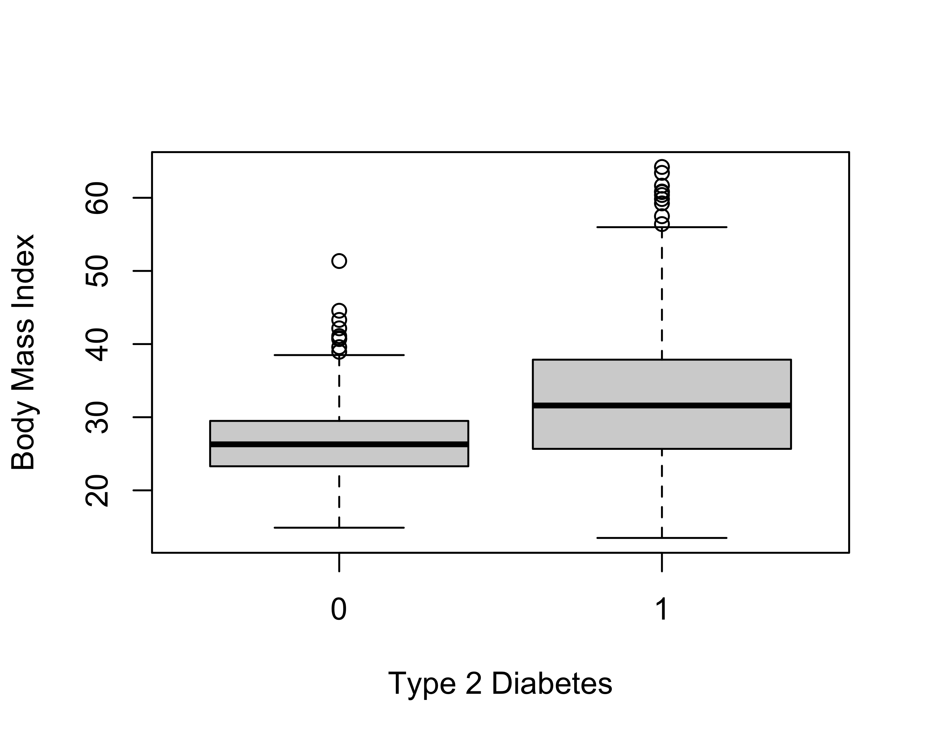
The @snps table now carries, for every marker, the call rate, the minor allele frequency (maf), the observed heterozygosity (hz) and the Hardy–Weinberg p-value (hwe). We summarise the autosomal markers:
    callrate           maf                hz              hwe
 Min.   :0.0000   Min.   :0.00000   Min.   :0.0000   Min.   :0.0000
 1st Qu.:0.9863   1st Qu.:0.05906   1st Qu.:0.1041   1st Qu.:0.2024
 Median :0.9884   Median :0.14271   Median :0.2406   Median :0.4709
 Mean   :0.9823   Mean   :0.18125   Mean   :0.2538   Mean   :0.4692
 3rd Qu.:0.9905   3rd Qu.:0.28638   3rd Qu.:0.4086   3rd Qu.:0.7353
 Max.   :0.9979   Max.   :0.50000   Max.   :0.5464   Max.   :1.0000
                  NAs    :2         NAs    :2        NAs    :2
Minor allele frequency measures how common the rarer allele is; markers that are (nearly) monomorphic carry almost no information. Hardy–Weinberg equilibrium relates genotype frequencies to allele frequencies in a large, randomly mating population; a strong departure often flags a genotyping error — or genuine biology such as selection or population structure. Count the markers that fail typical thresholds:
     monomorphic     low_callrate hwe_p_below_1e_6
               1               76              337
You can compare the HWE distribution between the two populations (diabetes / no diabetes) by re-computing it within each group:
controls    cases
61 360 Do you see a difference in the number of HWE-violating markers between the two populations? Can you explain why a population might be out of HWE?
The target phenotype (dm2) is binary, so a first association solution is a logistic regression per marker, adjusting for age, sex and BMI. gaston::association.test() does exactly this with response = "binary"; we pass the covariates (plus an intercept column) in X. We restrict the scan to individuals with complete covariates and to the autosomes.
[1] 7020The scan output has one row per marker with an association p-value. A Manhattan plot shows genome-wide significance (\(-\log_{10}\) p) along the genome (Figure 3.2):
manhattan(gwa1, pch = 16)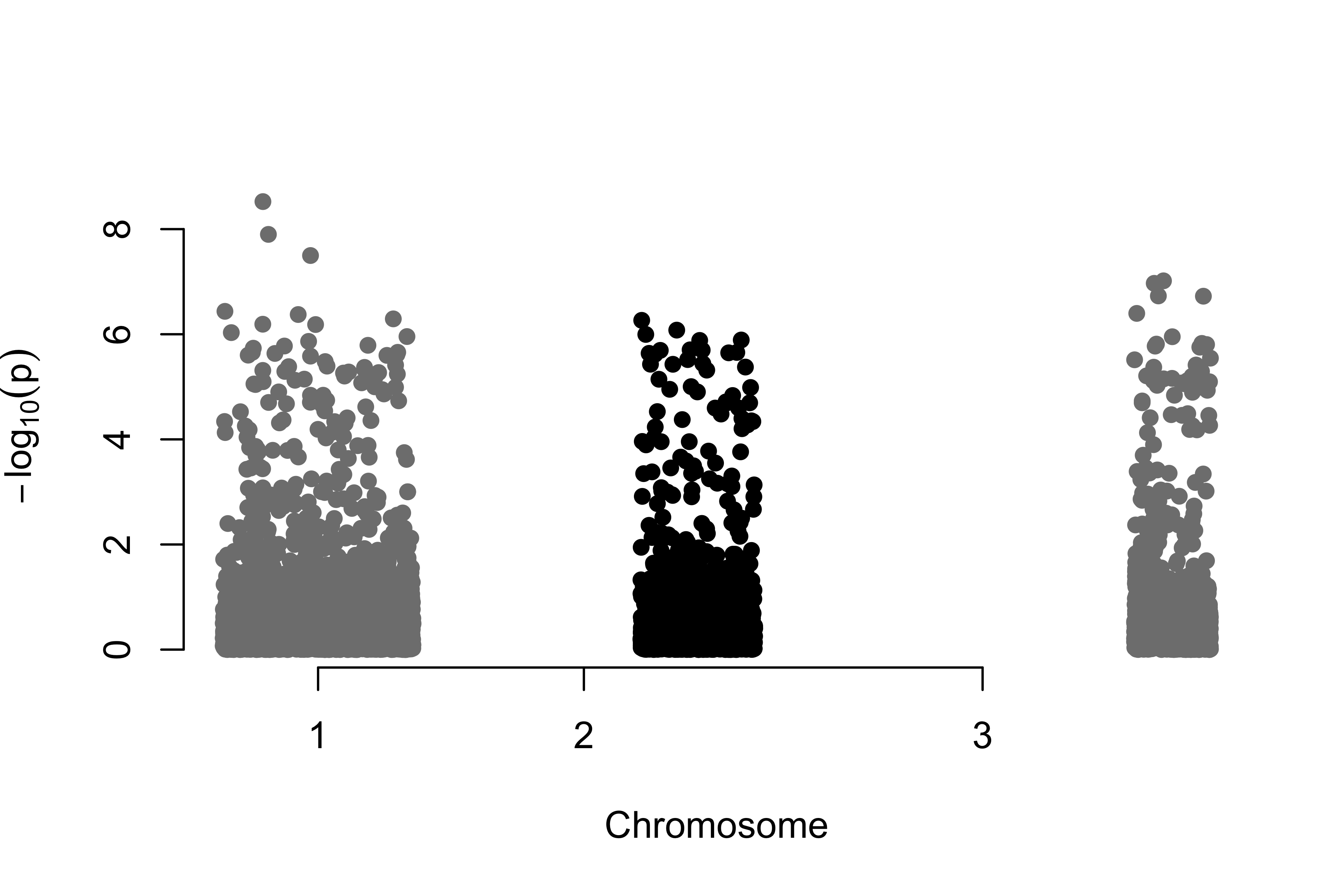
The most significant markers are ranked by p-value:
Before trusting any hit we check calibration with a QQ plot — observed \(-\log_{10}\) p-values against those expected under the null — and the genomic inflation factor \(\lambda\), the ratio of the observed median test statistic to its null expectation. \(\lambda \approx 1\) means confounding is under control; \(\lambda \gg 1\) signals population structure or genotyping artefacts inflating the whole scan (Figure 3.3).
qqplot.pvalues(gwa1$p)
title(sub = sprintf("Initial scan: lambda = %.2f", lambda1))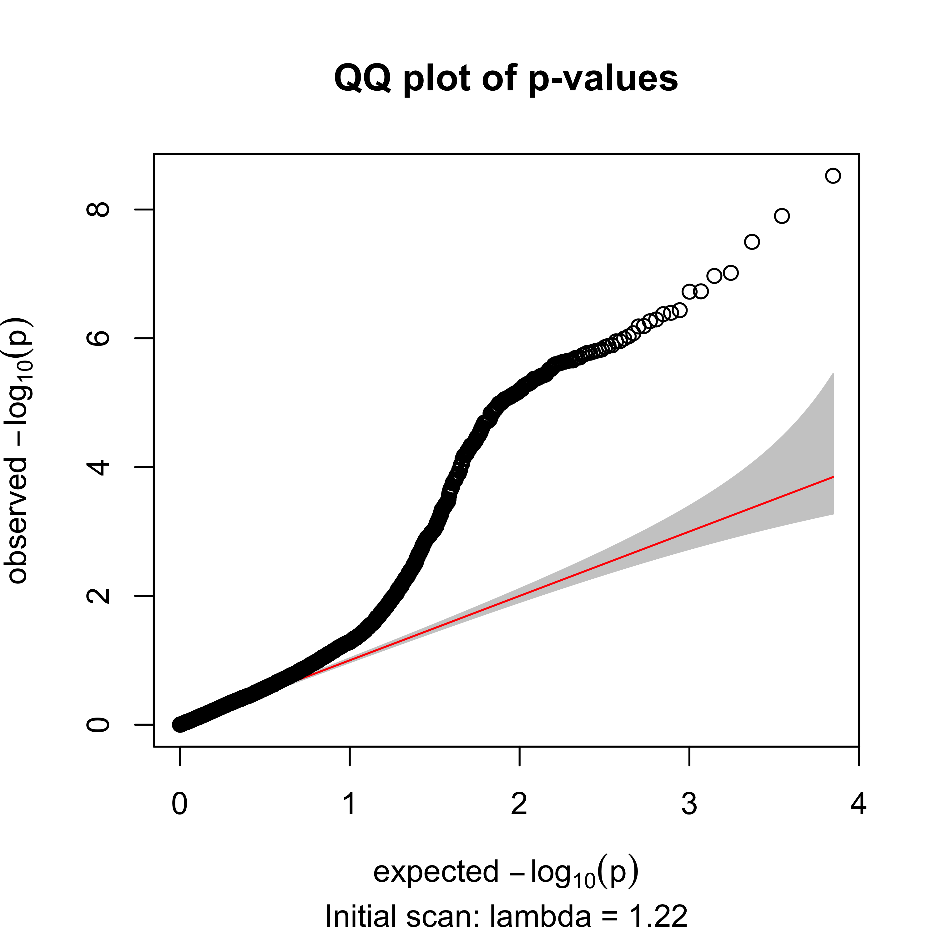
The inflation factor is \(\lambda = 1.22\) — above 1, a red flag that the raw scan is confounded (exactly what the quality control below will address).
With thousands of markers tested at once, an uncorrected \(p < 0.05\) yields hundreds of false positives. Judge hits against a genome-wide threshold — Bonferroni (\(0.05/m\) for \(m\) markers) or a controlled false-discovery rate (FDR, Benjamini–Hochberg via p.adjust(gwa1$p, "BH")).
Can you find whether any of the markers in the table have a clinical relationship? What genome-wide significance threshold would you use for \(m\) markers?
The odd HWE distribution and probable genotyping errors are blinding our analysis. Before a second scan we clean the dataset. We drop markers with a low call rate, a very low minor allele frequency, or a gross HWE violation, and we drop individuals with a low call rate or extreme genome-wide heterozygosity (a classic signal of sample contamination or poor DNA quality).
autosomal_markers           pass_qc
7020 6389 individuals low_callrate het_outliers pass_qc
950 4 8 938 Next we look for genetic outliers — a hidden subpopulation that, mixed with the rest, inflates the whole scan. We build the genetic relationship matrix (GRM) from common autosomal markers and take its leading principal components: individuals cluster by ancestry along the first PCs.3 Figure 3.4 shows the result.
gc <- geno[ok, auto & geno@snps$maf > 0.05 & geno@snps$callrate > 0.95]
standardize(gc) <- "p"
K   <- GRM(gc)
pcs <- eigen(K, symmetric = TRUE)$vectors[, 1:2]
colnames(pcs) <- c("PC1", "PC2")
km  <- kmeans(pcs, centers = 2, nstart = 50)
major <- as.integer(names(which.max(table(km$cluster))))
table(cluster = km$cluster)
cluster
1 2
923 25 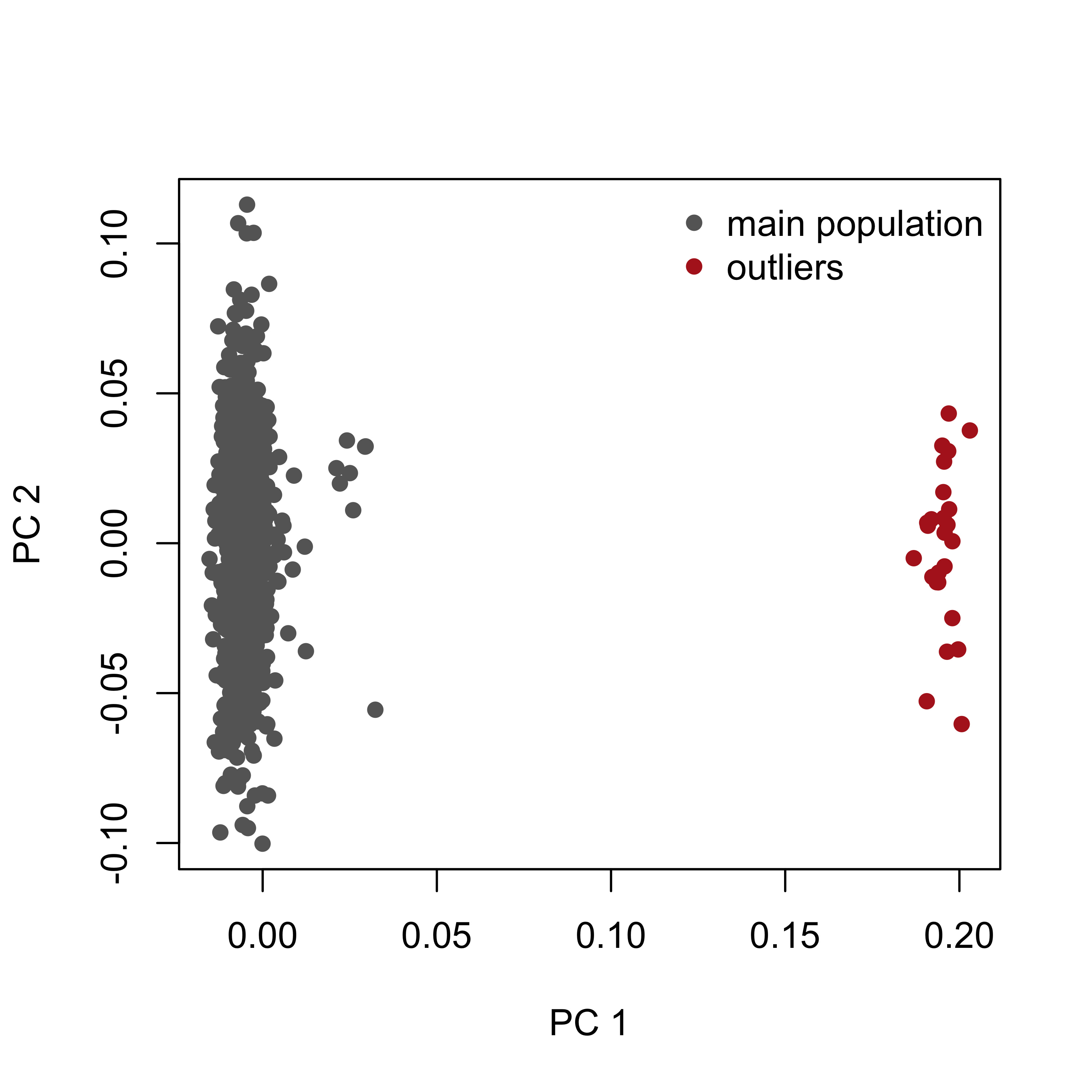
The minor cluster is discarded as an outlier population, as can be understood graphically from Figure 3.4.
An alternative to removing the outliers is to keep everyone and add the leading principal components as covariates in the association model (X = cbind(1, PC1, PC2, age, sex, bmi)). Both strategies control the stratification; here we remove the small outlier cluster so the effect on \(\lambda\) is easy to see.
dm2. Does the minor cluster correspond to cases, controls, or neither?geno@snps$chr == "X", compute per-individual X heterozygosity and look for mismatches. Why is this an important QC step?dm2 it contains both cases and controls. So it confounds (stratifies) the scan rather than being the biological signal.We now assemble the clean dataset: the individuals in the main cluster that also pass the per-individual QC, and the markers that pass the per-marker QC.
With the dataset clean — free of the stratified outliers, low-quality markers and individuals — we re-run the genome-wide scan against the type 2 diabetes phenotype (Figure 3.5):
Xc2  <- cbind(1, pheno_qc$age, pheno_qc$sex, pheno_qc$bmi)
gwa2 <- association.test(geno_qc, Y = pheno_qc$dm2, X = Xc2,
                         method = "lm", response = "binary", test = "wald")
lambda2 <- genomic_lambda(gwa2$p)manhattan(gwa2, pch = 16)
Compare these results with the first markers from the Section 3.2.1.
Re-checking calibration after QC, the inflation should have fallen back towards 1 (Figure 3.6):
qqplot.pvalues(gwa2$p)
title(sub = sprintf("After QC: lambda = %.2f", lambda2))
Inflation dropped from \(\lambda = 1.22\) (initial) to \(\lambda = 1.01\) after QC: removing the stratified outliers and bad markers de-confounded the scan. The strongest surviving hit is rs7903146, a variant in the TCF7L2 gene and the best-established common risk allele for type 2 diabetes — a reassuring positive control.
association.test, the GRM, and the mixed models used next.Worked solutions for the exercises are in the collapsed callouts below each exercise.
Write a laboratory report following the structure of this text. It should contain an introduction, the goals of each section, and a description of the results of each part. Include any graphics relevant to making your work understandable. The lab should be delivered within two weeks.
Earlier editions of this lab used GenABEL (descriptives.marker, qtscore, check.marker, ibs); GenABEL has since been archived from CRAN. gaston reads the same data in PLINK bed format and provides the equivalent building blocks — per-marker and per-individual statistics, a genetic relationship matrix (GRM) for stratification, and a per-marker association test — which is what we use here.↩︎
ge03d2 is the simulated type-2-diabetes example that shipped with the GenABEL “getting started with GWA” tutorial (package GenABEL.data). Because GenABEL is archived, we exported it once to PLINK bed format with scripts/make-ge03d2-bed.R and committed the result, so the lab reads it with gaston and never loads GenABEL. Provenance and archived sources: GenABEL.data on the CRAN archive, the GenABEL archive, and Aulchenko et al. (2007), Bioinformatics 23(10):1294–1296.↩︎
This replaces the older Identity-By-State + multidimensional-scaling recipe. Both project a matrix of genetic similarity between every pair of individuals into a few dimensions; the eigendecomposition (PCA) of the GRM is the modern standard and is what tools such as PLINK and EIGENSTRAT use.↩︎