Time-Series & Sequence Modeling with RNNs

Advanced Topics in Machine Learning for Bioinformatics and Biomedical Engineering

Joana Gelabert

joana.gelabert.xirinachs@upc.edu

Universitat Politècnica de Catalunya - BarcelonaTech

b2slab | Institut de Recerca i Innovació en Salut (IRIS)

Dr. Alexandre Perera Lluna

Alexandre.Perera@upc.edu

Universitat Politècnica de Catalunya - BarcelonaTech

b2slab | Institut de Recerca i Innovació en Salut (IRIS)

April 20, 2026

Introduction: Sequence Models for Bioinformatics

Why sequence models?

Most biologically meaningful information is carried in ordered sequences, not in flat feature vectors.

Learning goals

1. Recognise the sequential structure of core biological data types.
2. State the modelling requirements that arise from variable-length, ordered input.
3. Identify the two fundamental limitations of MLPs on sequence data.
4. Explain why those limitations motivate dedicated sequence architectures.

This section sets the problem. Students should leave knowing why standard MLPs are insufficient before we introduce the first recurrent architecture. The argument is not that MLPs are wrong; it is that their inductive biases do not match the structure of sequence data.

Why sequence models?

Biological sequences are everywhere:

• DNA: ATCGATCGTA…
• Proteins: MKTAYIAKQR…
• ECG: \(x_1, x_2, \ldots, x_T\)
• EEG signals over time
• Gene expression time-courses

Figure 1: Simulated ECG signal at 110 bpm, with labelled P, Q, R, S, T waves.

The biological world is sequential

Biological function is encoded in the order of discrete or continuous measurements taken over time or position.

• Genome: linear string of nucleotides; regulatory elements depend on precise arrangement
• Transcriptome: spliced mRNA sequences; reading frame determines the amino acid coded at every position
• Proteome: amino acid chain whose fold is determined by residue sequence
• Omics time series: gene expression or metabolite levels measured at successive time points
• Clinical signals: ECG traces, longitudinal lab values, patient event histories
• Clinical text: Electronic health records, discharge summaries, and radiology reports

Emphasise that in each case reordering the elements changes the biology. A scrambled promoter no longer binds its transcription factor. A scrambled protein no longer folds. This is the qualitative argument for why order-aware models are necessary.

Sequential biological data: four modalities

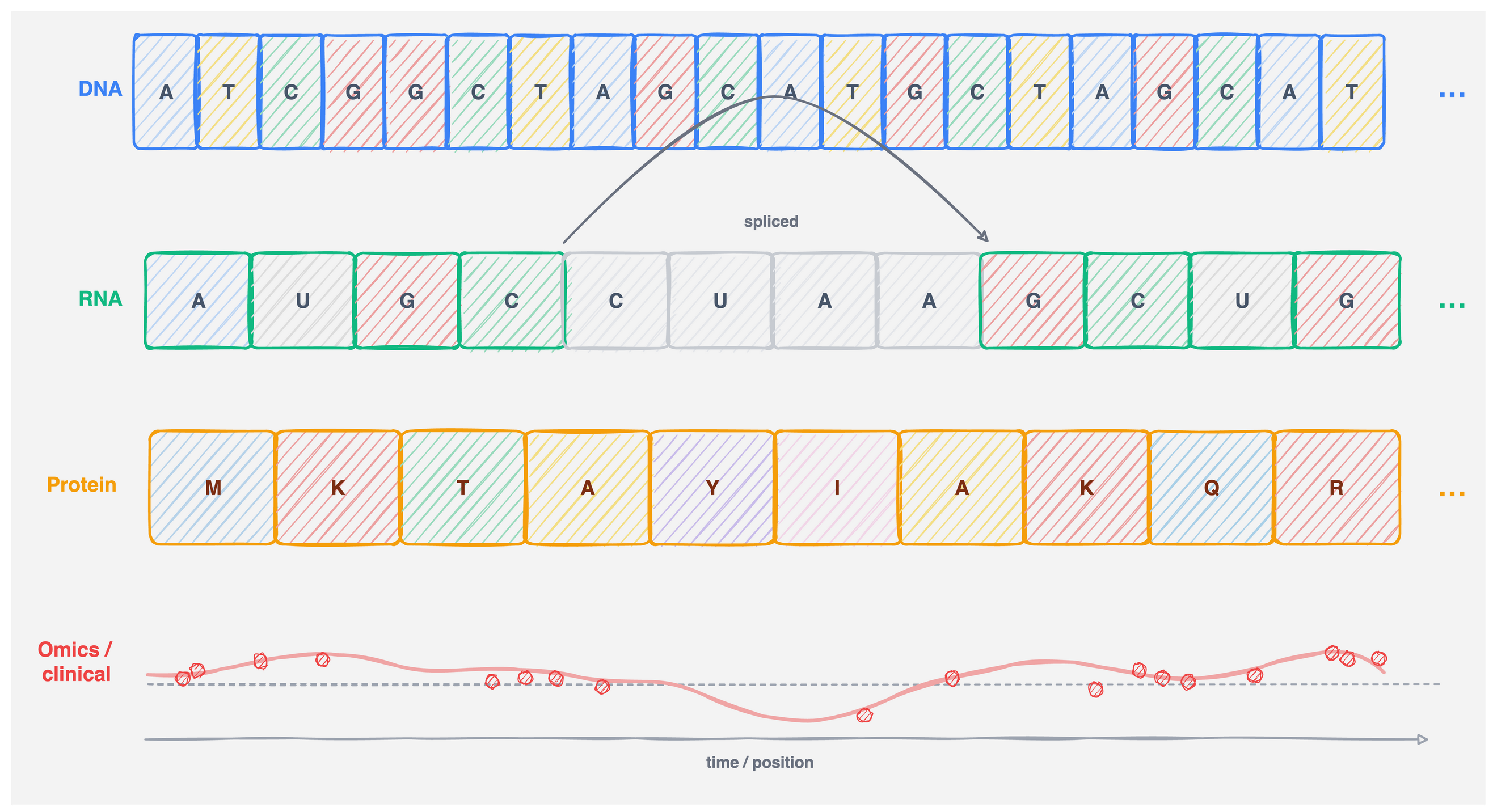
Figure 2: Four sequential modalities encountered in bioinformatics. Each row represents one data type; the horizontal axis is always position or time.

Walk through each lane briefly. Stress that the horizontal axis always encodes order: genomic position, transcript coordinate, residue index, or measurement time. The figure is not decorative; it is an argument for why position matters.

DNA and RNA: ordered nucleotide alphabets

A DNA or RNA sequence is a string over a small finite alphabet:

• DNA: \(\{A, T, C, G\}\), RNA (mRNA): \(\{A, U, C, G\}\)

Each position \(t\) carries a symbol \(x_t \in \mathcal{V}\), typically encoded as a one-hot vector \(x_t \in \{0,1\}^{|\mathcal{V}|}\).

Key properties that require order-awareness:

• Codons are non-overlapping triplets; reading frame depends on start position
• Splice sites are defined by short consensus sequences at precise locations
• Promoters and enhancers act through specific motifs embedded in context
• Distance between elements (e.g., TATA box to transcription start) is functionally relevant
• General annotations on the genome, such as ENCODE regulatory elements (ENCODE Project Consortium 2012).

Mention that in practice sequences are first embedded rather than kept as one-hot vectors. We will return to embeddings when we discuss transformers. The codon / reading-frame example is a clean, concrete illustration of why shuffling destroys biological meaning.

Proteins: function encoded in residue sequence

A protein is a sequence of amino acids over an alphabet of 20 standard residues, \(x_t \in \mathcal{V}_{\text{aa}}\) with \(|\mathcal{V}_{\text{aa}}| = 20\).

• Primary structure (the sequence) determines all higher-order structure under physiological conditions (Anfinsen 1973)
• Domains are compact functional units; their boundaries are sequence-defined
• Active sites depend on residues that may be far apart in the sequence but close in 3D space – a long-range dependency problem
• Sequence homology is used to infer function across species
• Structure prediction: predicting 3D protein structure from sequence alone reached near-experimental accuracy for many targets with AlphaFold2 (Jumper et al. 2021)

Downstream tasks include contact map prediction, variant effect scoring, and subcellular localisation.

The active site example is a concrete illustration of why long-range context matters: two residues 200 positions apart in sequence can sit 3 angstroms apart in 3D and catalyse the reaction together. A model that only looks locally will miss this.

Omics time series and clinical signals

Not all sequential data in bioinformatics is discrete or genomic.

• Bulk RNA-seq time courses: gene expression measured at \(T\) time points; \(x_t \in \mathbb{R}^{d_{\text{genes}}}\), often \(d > 10{,}000\)
• Single-cell trajectory inference: ordered pseudo-time series of cell states along a differentiation path
• Metabolomics and proteomics time series: continuous concentration profiles during a perturbation or disease progression
• EHR longitudinal data: irregularly sampled lab values, diagnoses, and drug events for each patient; \(T\) varies across patients
• Electrophysiology: continuous voltage signals (EEG, local field potential) sampled at kHz rates

Common challenges: irregular sampling, missing values, very long \(T\), and patient-level variability in length.

Contrast discrete symbol sequences (fixed alphabet) with continuous time series. The modelling choices differ: embeddings for symbols, direct real-valued input for continuous signals. Both share the variable-length and ordering challenges.

What defines a sequence modelling problem?

Three properties jointly distinguish sequence problems from standard supervised learning:

Order matters:

The output changes if the input is permuted. \(f(x_1, x_2) \ne f(x_2, x_1)\) in general. A bag-of-words or feature-vector model ignores this.

Length is variable:

Different instances have different \(T\). A single fixed architecture must handle all lengths without retraining.

Long-range dependencies:

The label at position \(t\) can depend on context far back (or ahead) in the sequence – dependencies may span hundreds or thousands of positions.

These three properties are not independent: handling variable length and long range simultaneously is the central challenge that motivates sequence-specific architectures.

This slide formalises the intuition from the previous slides. Write the three properties on the board and ask students to match them to a concrete biological example from each modality.

The MLP as a baseline

Recall the standard MLP: a composition of affine maps and nonlinearities.

For a single input \(\mathbf{x} \in \mathbb{R}^d\) and layer \(\ell\) out of \(L\) layers:

\[ \mathbf{h}^{(0)} = \mathbf{x}, \qquad \mathbf{h}^{(\ell)} = \phi\!\left(W^{(\ell)} \mathbf{h}^{(\ell-1)} + \mathbf{b}^{(\ell)}\right), \qquad \hat{y} = W^{(L)} \mathbf{h}^{(L-1)} + \mathbf{b}^{(L)} \]

The MLP is a universal approximator (Hornik et al. 1989) and the workhorse of most non-sequential tasks.

Where MLPs work well in bioinformatics:

• Fixed-size tabular inputs (gene expression matrices, k-mer count vectors)
• Classification of fixed-length feature representations
• Final prediction head on top of a learned representation

We are not dismissing MLPs. The goal is to show precisely where they fall short so that the motivation for RNNs (and later transformers) is unambiguous. Many real bioinformatics pipelines combine an upstream sequence encoder with an MLP prediction head.

MLP limitation 1: fixed input size

Fixed Input Size

An MLP with input layer of width \(d\) requires every input to have exactly \(d\) features. There is no mechanism to handle variable-length sequences natively.

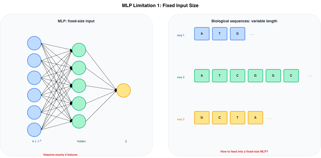
Figure 3: Left: an MLP requires exactly d input features. Right: biological sequences come in variable lengths — three sequences of lengths 3, 8 and 4 cannot share the same fixed-width input layer.

Fixed Input Size

The two engineering workarounds both lose information:

• Truncation: discard positions beyond a fixed cutoff – relevant context is dropped
• Padding + flattening: pad short sequences to length \(T_{\max}\) – the model must waste capacity learning to ignore padding

Figure 4: MLP fixed-size input vs variable-length sequences.

Ask students: if we pad all sequences to the length of the longest, what happens when we encounter a test sequence longer than any training sequence? The model has never seen inputs beyond that width. This is a practical failure mode, not just a theoretical one.

MLP limitation 2: no memory across positions

Even if we fix the length problem – e.g., by applying an MLP independently at each position)– the MLP has no way to pass information from one position to the next.

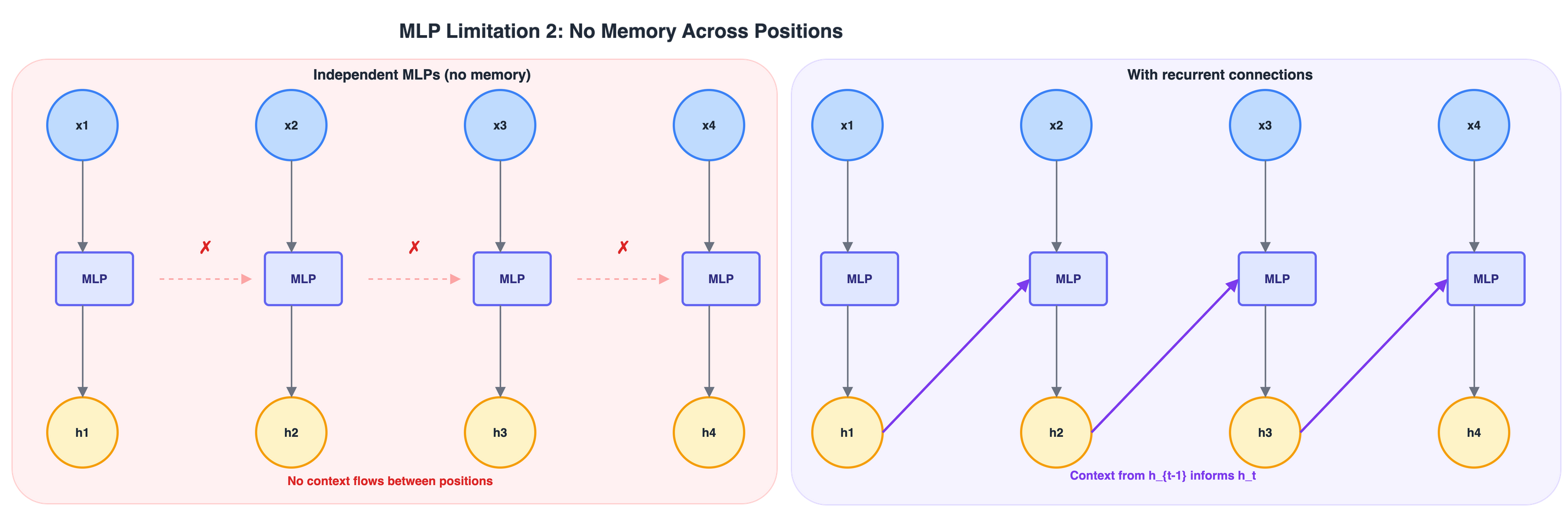
Figure 5: Left: independent MLPs applied at each position share no information (\(\times\)). Right: recurrent connections allow context from \(h_{t-1}\) to influence \(h_t\) (purple arrows).

The right panel is a preview, not a definition. Students do not need to know yet how the recurrent connection is computed. The point is only that the connection exists and is absent in the MLP case. The formal definition of an RNN comes in the next section.

MLP limitation 2: consequences for biology

For example, an MLP applied position-by-position cannot:

• Detect a motif that spans multiple positions without seeing all positions simultaneously (defeats variable-length handling)
• Track codon reading frame – the interpretation of position \(t\) depends on \(t \bmod 3\), which requires knowing where the sequence started
• Model splice site context – both the donor and acceptor site must be jointly considered, though they are tens to thousands of nucleotides apart
• Capture promoter–TSS distance – a regulatory element’s effect depends on its distance from the transcription start, not on its local identity alone

Houston, we have a …

This slide converts the abstract limitation into concrete biological failure modes. It answers the question students will ask: “Can’t we just concatenate everything and pass it to a big MLP?”

Providing the full flattened sequence as one input vector is not a solution: it fixes the length problem but creates a parameter matrix that grows as \(O(T \cdot d_{\text{in}})\), does not generalise to new lengths, and treats every position pair as equally related.

What a sequence model must provide

A model suited to sequential biological data needs at least four properties:

Property	Requirement
Variable-length input	Same parameters for any \(T\)
Position awareness	Representations respect order
Context propagation	Information at \(t\) influences representations at \(t' > t\)
Parameter efficiency	Parameters do not grow with \(T\)

Models we will study in this course, in order of increasing capacity:

• Recurrent Neural Networks (RNN): sequential hidden state; \(h_t = f(x_t, h_{t-1})\)
• Long Short-Term Memory (LSTM): gated memory cell; selectively retains long-range context
• Convolutional sequence models: parallel local context; used in motif detection, as seen in the previous CNN lecture
• Transformers and attention: all-pairs context; the basis of protein language models

This slide is a roadmap. Students should be able to look back at it at the end of the course and confirm that each architecture addresses the limitations identified here. The table is intentionally concise; each row will be unpacked in its own lecture.

Sequence Modelling Basics

The sliding window

Before recurrent networks, the standard approach was a sliding window: extract a fixed-width context of \(k\) positions around each target position and apply an MLP to that window.

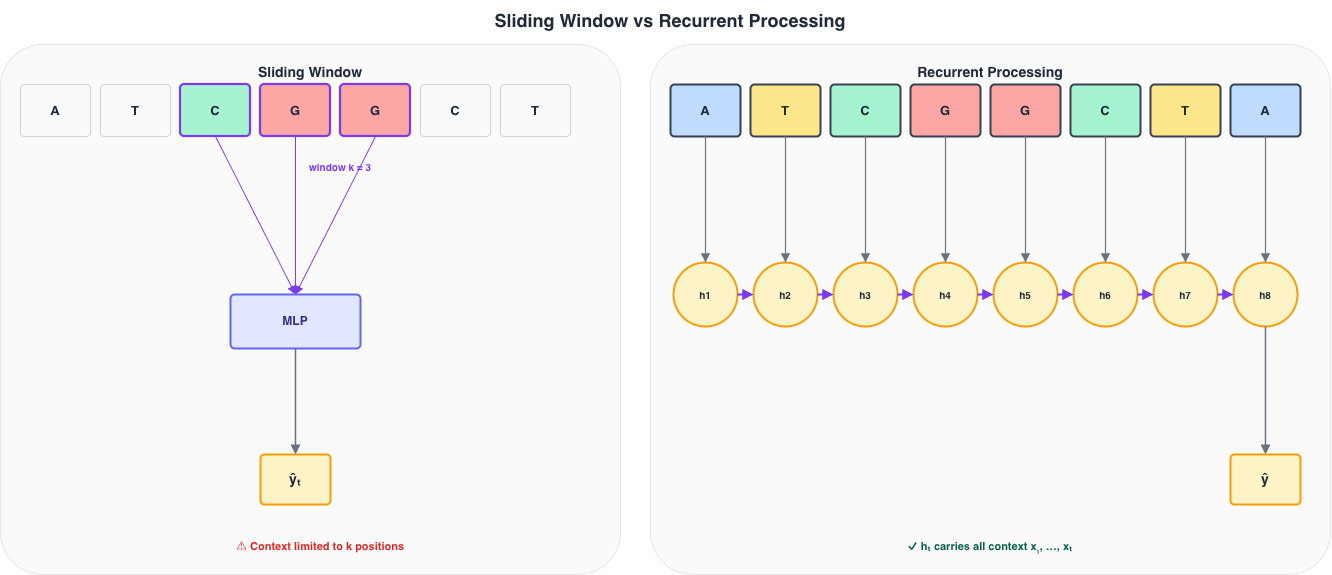
Figure 6: Left: a sliding window of size k=3 extracts a local context and applies an MLP. Right: a recurrent model accumulates all past context in h_t without a fixed horizon.

The sliding window was the backbone of early splice-site and promoter predictors such as NetGene2 and NNPP. Students from bioinformatics may have encountered these tools. The window is still used in CNNs for motif detection; the limitation addressed here is specifically about long-range context.

Sliding window: properties and limits

For a window of size \(k\) centred at position \(t\), the input to the MLP is:

\[ \mathbf{v}_t = \bigl[x_{t - \lfloor k/2 \rfloor}, \;\dots,\; x_t, \;\dots,\; x_{t + \lfloor k/2 \rfloor}\bigr] \in \mathbb{R}^{k \cdot d_{\text{in}}} \]

Strengths:

• Simple to implement; fully parallelisable across positions
• Captures local motifs (e.g., TATA box, splice consensus) efficiently
• Still used in convolutional layers as a learned multi-scale window

Limitations:

• Hard context horizon: positions more than \(k/2\) steps away are invisible
• Boundary artefacts: positions near the start or end of the sequence need padding
• No global state: the model cannot detect that a motif seen at position 20 is relevant to the label at position 200
• Width is a hyperparameter: too small misses context; too large inflates input dimensionality and makes the MLP expensive

The last bullet is a real practical issue. For protein contact prediction, relevant pairs can be 300 residues apart. A window wide enough to capture this would have input dimension \(300 \times 20 = 6000\) – and most of that window would be irrelevant for most positions.

Sequence modelling

• Sequence models differ in what they predict and when.
• The choice of task setting determines
  • the loss,
  • the output layer, and
  • how we read off predictions at inference time.

Sequence mapping

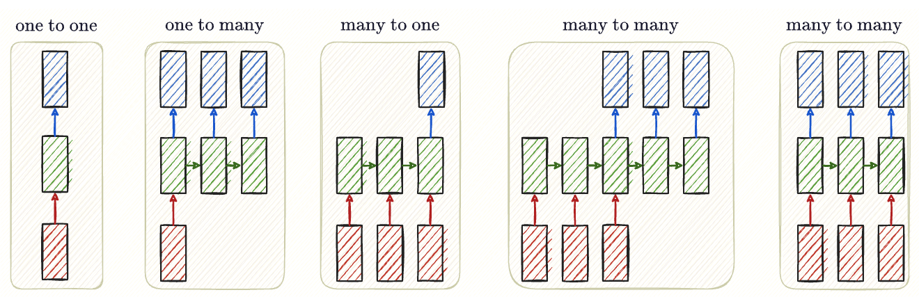
Generally, we will find these sequence mapping variants

Sequence task settings

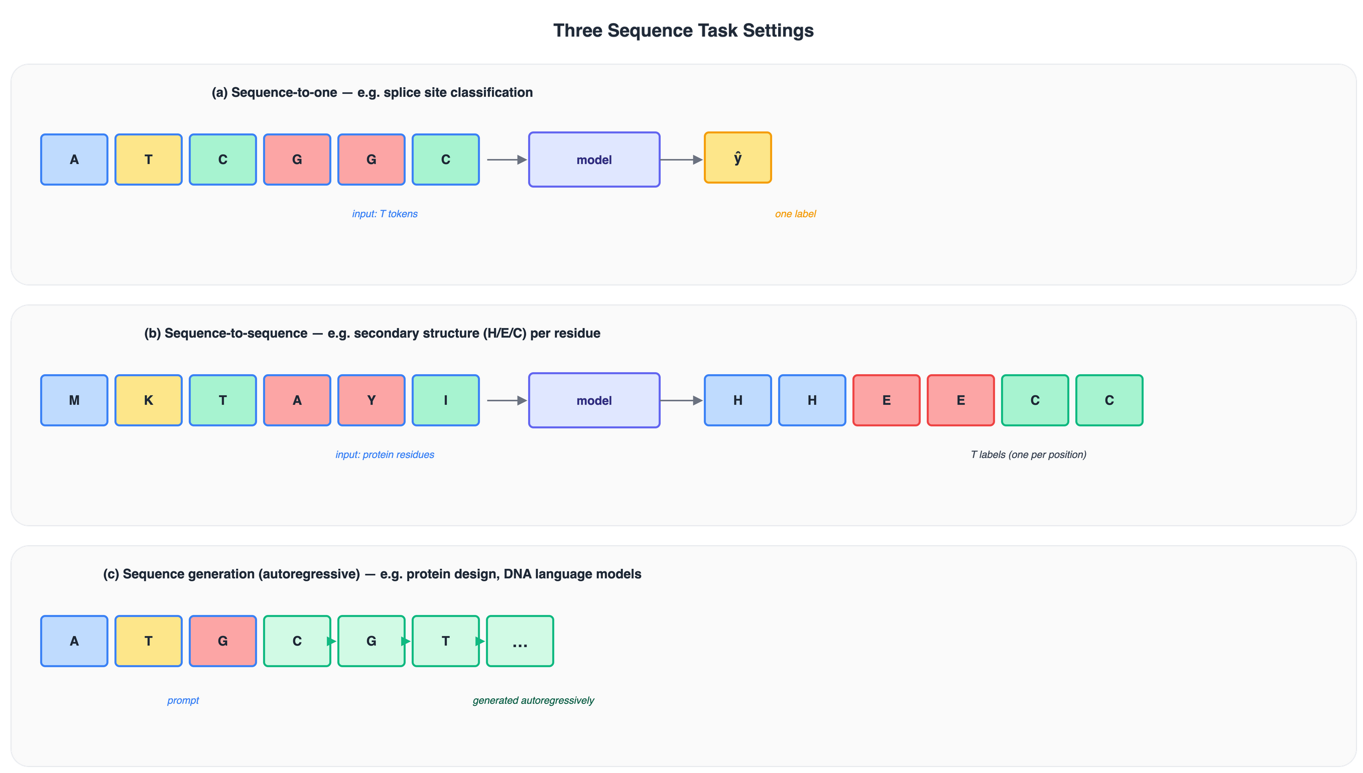
Figure 7: Three standard sequence task settings. (a) One label for the whole sequence. (b) One label per position. (c) Tokens generated one at a time, each conditioned on all previous tokens.

Walk through each row and make sure students can map a familiar task to each setting before moving on. The key distinction between (b) and (c): in sequence-to-sequence the target is determined by the input; in autoregressive generation the model produces its own input for the next step.

Sequence-to-one

A single label is produced for the entire input sequence of length \(T\).

\[ f_\theta : \mathbb{R}^{T \times d_{\text{in}}} \longrightarrow \mathbb{R}^{k} \]

The model reads all \(T\) positions and emits one prediction vector.

Some examples:

• Promoter / enhancer classification from a fixed-length DNA window
• Splice site prediction: does this sequence contain a donor or acceptor?
• Protein family classification from the full amino acid sequence
• Virulence or antibiotic resistance prediction from a gene sequence
• Patient-level outcome prediction from a longitudinal EHR record

Sequence-to-sequence

A label is produced at every position in the input sequence.

\[ f_\theta : \mathbb{R}^{T \times d_{\text{in}}} \longrightarrow \mathbb{R}^{T \times k} \]

The output has the same length \(T\) as the input; labels are aligned position by position.

Some examples:

• Secondary structure prediction: helix / sheet / coil label per residue
• Intrinsic disorder prediction: probability of disorder at each residue
• CpG island annotation: methylation state per cytosine position
• Named entity recognition in clinical text: drug / disease / dosage per token
• Base-calling from raw nanopore signals: nucleotide label per signal sample

The shared output head is important: the same linear layer is applied at every position. This is another instance of parameter sharing, extending the idea that we will introduce formally in the next few slides.

Sequence generation (autoregressive)

The model generates one token at a time, conditioning on all previously generated tokens.

\[ p(x_1, \dots, x_T) = \prod_{t=1}^{T} p\!\left(x_t \mid x_1, \dots, x_{t-1}\right) \]

At each step the model samples the next token, then feeds it back as input.

Some examples:

• Protein sequence design: generate amino acid sequences compatible with a target fold or function (Madani et al. 2023)
• DNA language models: predict the next nucleotide given genomic context
• scRNA-seq data augmentation: generate plausible synthetic expression profiles

This is the same principle used in large language models. The only difference in biology is that the vocabulary is small (\(|\mathcal{V}| = 4\) or \(20\)) but the sequences can be very long.

The factorisation on this slide is the chain rule of probability, not an assumption. It holds for any joint distribution. The autoregressive model estimates each conditional in the product. Make sure students are comfortable with the idea of feeding generated tokens back as inputs.

Recurrent processing: the key idea

A recurrent model maintains a hidden state \(h_t\) that is updated at every step:

\[ h_t = f\!\left(x_t,\, h_{t-1}\right) \]

• \(h_t \in \mathbb{R}^{d_h}\) is a fixed-size summary of all past input \(x_1, \dots, x_t\), \(h_0 \in \mathbb{R}^{d_h}\) is an initial state (typically \(\mathbf{0}\))
• \(f\) is the same function applied at every step (defined by learned parameters) .

Recurrent processing: the key idea

A recurrent model maintains a hidden state \(h_t\) that is updated at every step:

\[ h_t = f\!\left(x_t,\, h_{t-1}\right) \]

Three consequences that directly address the MLP limitations:

• Unbounded context: \(h_t\) can in principle depend on \(x_1\), however far back
• Variable-length input: the same recurrence runs for any \(T\)
• Fixed parameter count: the size of the model does not grow with \(T\)

The gradient signal must propagate through many time steps to update weights that influenced early states, –> vanishing gradient problem – the main motivation for LSTMs and GRUs.

Do not define \(f\) in detail here. The point of this slide is the principle: a fixed-size state is updated at every step. The specific form of \(f\) (tanh, gates, etc.) is the content of the RNN and LSTM lectures.

Parameter sharing across time

The function \(f\) uses the same parameters at every time step. For the simplest recurrent model:

\[ h_t = \phi\!\left(W_x\, x_t + W_h\, h_{t-1} + b\right) \]

where \(W_x \in \mathbb{R}^{d_h \times d_{\text{in}}}\), \(W_h \in \mathbb{R}^{d_h \times d_h}\), and \(b \in \mathbb{R}^{d_h}\) are shared across all \(T\) steps.

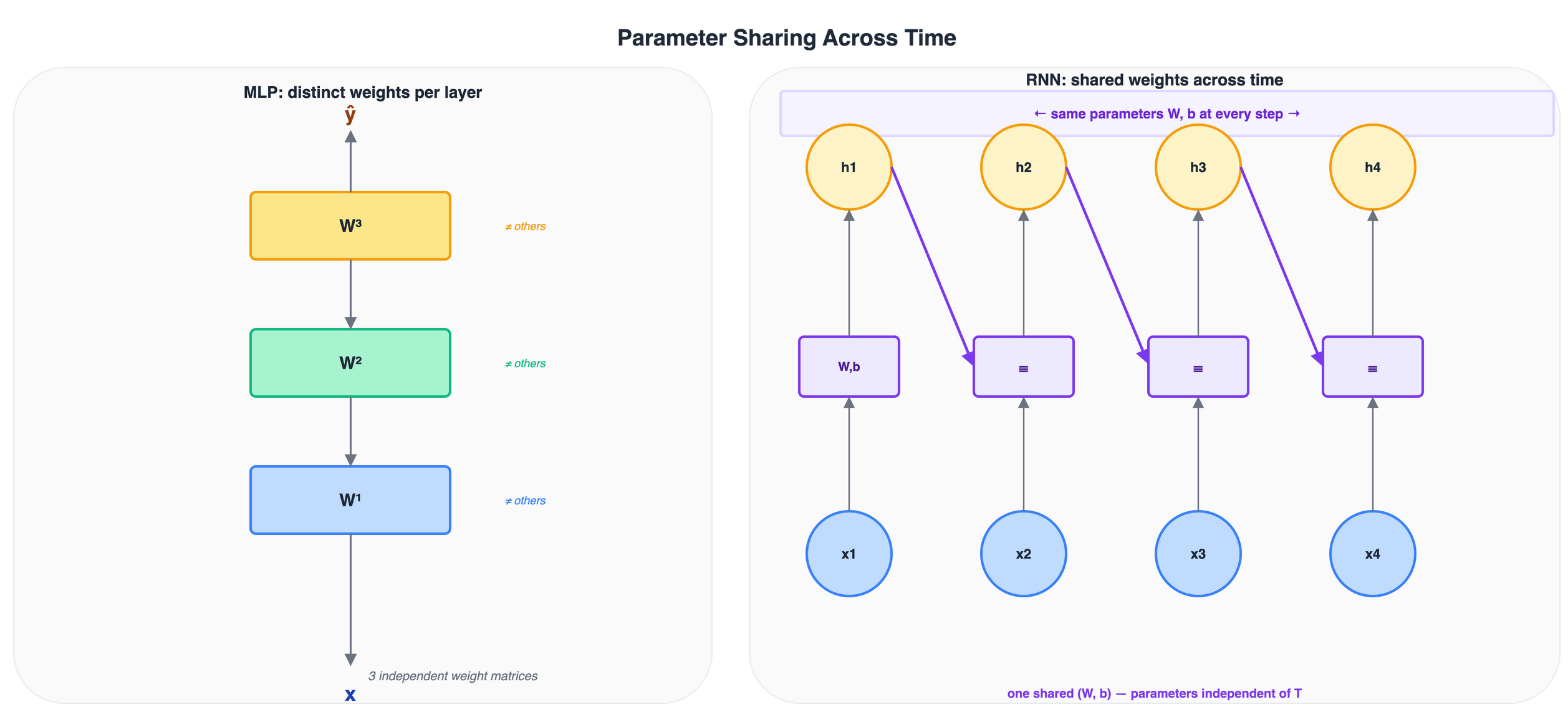
Figure 8: Left: an MLP uses distinct weight matrices at each layer. Right: a recurrent model reuses the same (W, b) at every time step, keeping the parameter count independent of sequence length T.

Why parameter sharing matters

Sharing parameters across time has two important consequences.

Generalisation to unseen lengths

The model is trained on sequences of length up to \(T_{\max}\), but the same recurrence \(h_t = f(x_t, h_{t-1})\) can be unrolled for any \(T\) at test time. No architecture change or retraining is required.

Regularisation by structure

Using the same \(W_x\), \(W_h\), \(b\) everywhere forces the model to learn a universal rule for updating context – not a position-specific rule. This reduces the effective number of parameters from \(O(T \cdot d_h^2)\) to \(O(d_h^2)\).

Note

Parameter sharing is the same principle as weight tying in convolutional networks: a filter is applied at every spatial position. In RNNs the axis of sharing is time rather than space.

The connection to CNNs is worth drawing explicitly: students who have seen convolutional filters should recognise the analogy immediately. The key difference is that CNNs apply the same filter to a fixed-size window in parallel, whereas RNNs pass context forward sequentially.

Recurrent neural networks

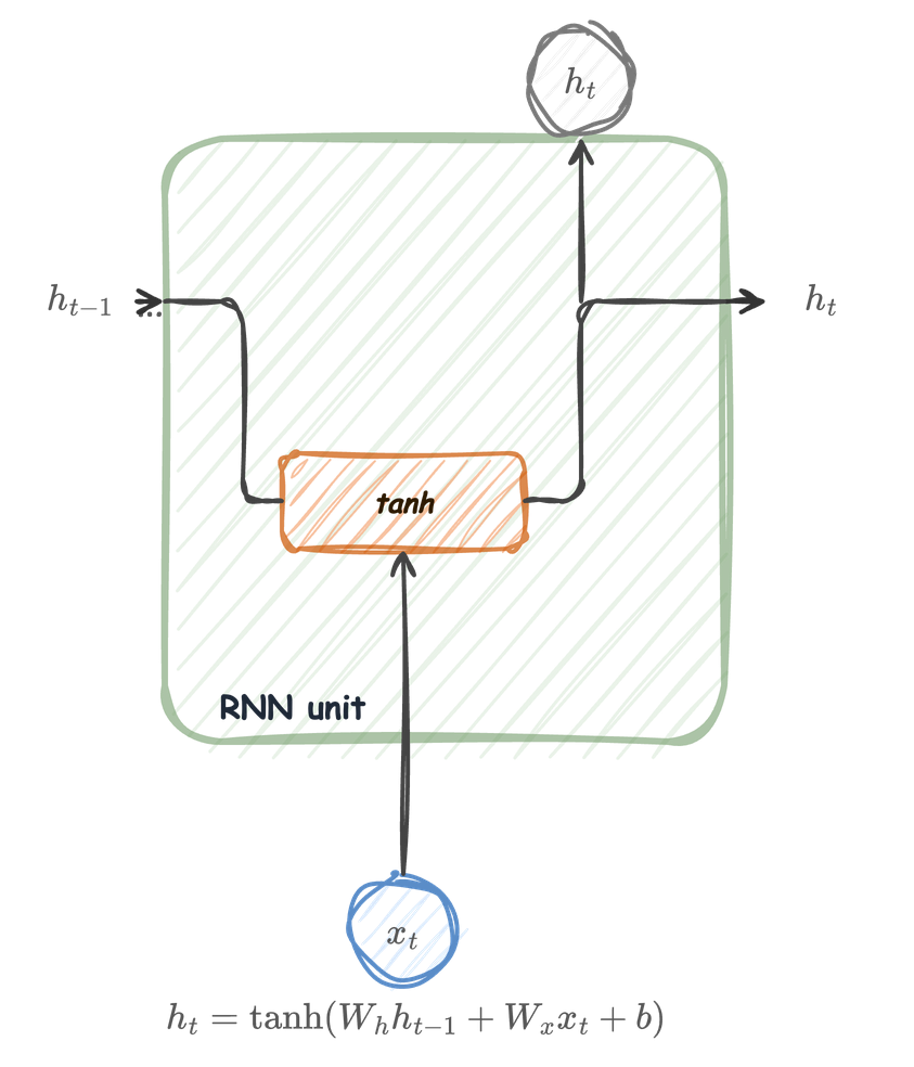
The RNN unit

At each time step \(t\), the unit receives two inputs:

• \(x_t \in \mathbb{R}^{d_{\text{in}}}\) — the current observation
• \(h_{t-1} \in \mathbb{R}^{d_h}\) — the hidden state carried from the previous step

It produces a new hidden state:

\[ h_t = \tanh(W_h h_{t-1} + W_x x_t + b) \]

• \(W_h \in \mathbb{R}^{d_h \times d_h}\) mixes the recurrent memory
• \(W_x \in \mathbb{R}^{d_h \times d_{\text{in}}}\) projects the current input
• \(\tanh\) keeps values in \((-1, 1)\), preventing unbounded growth
• \(h_t\) is both the output at step \(t\) and the input to step \(t+1\)

RNN unit: \(h_{t-1}\) and \(x_t\) enter the tanh activation; \(h_t\) exits and is also fed back at the next step.

The RNN unit

Unfolded

The RNN unit animated

link

Hidden state as a lossy summary

The hidden state \(h_t\) compresses the entire history \((x_1, x_2, \dots, x_t)\) into a fixed-size vector.

\[ h_t = \tanh(W_h\, h_{t-1} + W_x\, x_t + b) \]

• At \(t=1\): \(h_1\) depends only on \(x_1\) (and the initial state \(h_0\), often zero)
• At \(t=T\): \(h_T\) must encode everything relevant from \(T\) steps

Note

The representation is lossy: \(h_t\) has \(d_h\) entries regardless of how long the sequence is. Early inputs can only influence the output if their effect survives repeated multiplication and squashing through \(\tanh\).

Ask students: what happens if \(d_h\) is too small relative to sequence length? The network simply cannot remember enough. This is analogous to compressing a long DNA read into a fixed-length hash — at some point you lose information.

Output at each step

The hidden state \(h_t\) can be read out at every step or only at the end, depending on the task.

Sequence-to-sequence (e.g., per-residue secondary structure prediction):

\[ y_t = W_y\, h_t + b_y, \qquad t = 1, \dots, T \]

Sequence-to-one (e.g., classify a promoter sequence as active/inactive):

\[ y = W_y\, h_T + b_y \]

• \(W_y \in \mathbb{R}^{k \times d_h}\), \(b_y \in \mathbb{R}^{k}\) are the output-layer parameters
• \(k\) = number of output classes or targets
• The loss is computed on \(y_t\) (per step) or \(y\) (final), then backpropagated through the unrolled graph

Parameters are shared across time

A key property: \(W_h\), \(W_x\), and \(b\) are the same at every step.

• The RNN applies the same function \(f(h_{t-1}, x_t; \theta)\) at \(t=1, 2, \dots, T\)
• This means one set of parameters handles sequences of any length
• Gradients from every time step contribute to the same \(W_h\), \(W_x\), \(b\)

Tip

Weight sharing is what makes RNNs fundamentally different from a feed-forward network with \(T\) separate layers. It also makes gradient computation more involved, because changing \(W_h\) affects \(h_1\), which affects \(h_2\), and so on.

Backpropagation Through Time

From backprop to BPTT

In a feed-forward network, backprop walks backward through layers.

In an RNN, the computational graph is the unrolled chain \(h_1 \to h_2 \to \cdots \to h_T\).

Backpropagation Through Time (BPTT) is simply backprop applied to this unrolled graph (Werbos 1990):

1. Forward: compute \(h_1, h_2, \dots, h_T\) and the loss \(L\)
2. Backward: propagate \(\frac{\partial L}{\partial h_t}\) from \(t = T\) back to \(t = 1\)
3. Accumulate: sum the gradient contributions from every step into \(\frac{\partial L}{\partial W_h}\), \(\frac{\partial L}{\partial W_x}\), \(\frac{\partial L}{\partial b}\)

Note

BPTT is not a new algorithm. It is standard backprop on a graph that happens to repeat the same operation \(T\) times with shared weights.

The RNN unit animated

link

The chain rule through time

Consider a loss that depends only on the final state: \(L = \ell(h_T)\).

The gradient of \(L\) with respect to \(h_t\) (for \(t < T\)) requires chaining through every intermediate step:

\[ \frac{\partial L}{\partial h_t} = \frac{\partial L}{\partial h_T} \prod_{s=t+1}^{T} \frac{\partial h_s}{\partial h_{s-1}} \]

Each Jacobian factor comes from the recurrence \(h_s = \tanh(W_h\, h_{s-1} + W_x\, x_s + b)\):

\[ \frac{\partial h_s}{\partial h_{s-1}} = \mathrm{diag}\!\bigl(\tanh'(z_s)\bigr)\; W_h \]

where \(z_s = W_h\, h_{s-1} + W_x\, x_s + b\) and \(\tanh'(z) = 1 - \tanh^2(z)\).

The gradient is a product of many matrices

Expanding the product:

\[ \frac{\partial L}{\partial h_t} = \frac{\partial L}{\partial h_T} \prod_{s=t+1}^{T} \mathrm{diag}\!\bigl(1 - h_s^2\bigr)\; W_h \]

This is a product of \((T - t)\) matrices, all involving \(W_h\) (Pascanu et al. 2013).

• If \(T - t\) is large, this product can shrink to zero or blow up
• The behaviour depends on the spectral properties of \(W_h\) and the saturation of \(\tanh\)

Warning

This is the fundamental difficulty of training RNNs on long sequences: the gradient signal must survive many multiplicative steps to reach early time steps.

Gradient w.r.t. shared parameters

Since \(W_h\) appears at every step, the total gradient is a sum over time:

\[ \frac{\partial L}{\partial W_h} = \sum_{t=1}^{T} \frac{\partial L}{\partial h_t}\; \frac{\partial h_t}{\partial W_h}\bigg|_{\text{local}} \]

where the local term is:

\[ \frac{\partial h_t}{\partial W_h}\bigg|_{\text{local}} = \mathrm{diag}\!\bigl(1 - h_t^2\bigr)\; h_{t-1}^\top \]

The same pattern applies to \(W_x\) and \(b\). Each step contributes a term, and the difficulty lies in the factor \(\frac{\partial L}{\partial h_t}\), which requires the long product from the previous slide.

Why does diag() appear here?

The recurrence uses a vector activation:

\[ h_s = \tanh(z_s) \]

where \(z_s \in \mathbb{R}^{d_h}\). This means that \(\tanh\) is applied elementwise:

\[ h_{s,i} = \tanh(z_{s,i}) \qquad \text{for each } i = 1,\dots,d_h \]

So the Jacobian of \(h_s\) with respect to \(z_s\) has entries

\[ \left(\frac{\partial h_s}{\partial z_s}\right)_{ij} = \frac{\partial h_{s,i}}{\partial z_{s,j}} \]

• If \(i=j\), then \(\frac{\partial h_{s,i}}{\partial z_{s,i}} = \tanh'(z_{s,i})\)
• If \(i\neq j\), then \(\frac{\partial h_{s,i}}{\partial z_{s,j}} = 0\)

because coordinate \(h_{s,i}\) depends only on its own input \(z_{s,i}\).

The tanh Jacobian is diagonal

Therefore:

\[ \frac{\partial h_s}{\partial z_s} = \begin{bmatrix} \tanh'(z_{s,1}) & 0 & \cdots & 0\\ 0 & \tanh'(z_{s,2}) & \cdots & 0\\ \vdots & \vdots & \ddots & \vdots\\ 0 & 0 & \cdots & \tanh'(z_{s,d_h}) \end{bmatrix} = \operatorname{diag}\!\bigl(\tanh'(z_s)\bigr) \]

This is exactly the diag() term in the BPTT product.

The tanh Jacobian is diagonal

Then, since

\[ z_s = W_h h_{s-1} + W_x x_s + b \]

we also have

\[ \frac{\partial z_s}{\partial h_{s-1}} = W_h \]

and by the chain rule:

\[ \frac{\partial h_s}{\partial h_{s-1}} = \frac{\partial h_s}{\partial z_s} \frac{\partial z_s}{\partial h_{s-1}} = \operatorname{diag}\!\bigl(\tanh'(z_s)\bigr)\, W_h = \mathrm{diag}(1 - h_s^2)\; W_h \]

Tiny 2D example

Let

\[ z_s = \begin{bmatrix} z_1\\ z_2 \end{bmatrix}, \qquad h_s = \begin{bmatrix} \tanh(z_1)\\ \tanh(z_2) \end{bmatrix} \]

Then

\[ \frac{\partial h_s}{\partial z_s} = \begin{bmatrix} \frac{\partial \tanh(z_1)}{\partial z_1} & \frac{\partial \tanh(z_1)}{\partial z_2}\\[4pt] \frac{\partial \tanh(z_2)}{\partial z_1} & \frac{\partial \tanh(z_2)}{\partial z_2} \end{bmatrix} = \begin{bmatrix} \tanh'(z_1) & 0\\ 0 & \tanh'(z_2) \end{bmatrix} \]

So diag() is just a compact way to say:

each coordinate gets multiplied by its own \(\tanh'\) value, and there are no cross-terms between coordinates.

Note

In backprop code we rarely build this diagonal matrix explicitly. Multiplying by \(\operatorname{diag}(v)\) is usually implemented as an elementwise multiply by the vector \(v\).

Vanishing and exploding gradients

Why gradients vanish

Recall the product that links \(h_T\) back to \(h_t\):

\[ \prod_{s=t+1}^{T} \mathrm{diag}(1 - h_s^2)\; W_h \]

Vanishing occurs when the spectral norm of each factor is less than 1:

• \(\tanh'(z) \in (0, 1]\), and is close to 0 when \(|z|\) is large (saturation)
• If the largest singular value of \(W_h\) is moderate, each multiplication shrinks the gradient
• After many steps the gradient reaching early time steps is negligibly small

Consequence: the network cannot learn long-range dependencies. Parameters are updated based almost entirely on the last few steps.

Why gradients explode

Exploding occurs when the spectral norm of \(W_h\) is large enough that the product grows exponentially:

\[ \left\| \prod_{s=t+1}^{T} \mathrm{diag}(1 - h_s^2)\; W_h \right\| \;\approx\; \rho^{T-t} \]

where \(\rho\) is an effective per-step amplification factor.

• Even \(\rho = 1.1\) gives \(1.1^{50} \approx 117\) after 50 steps
• Gradients become extremely large, causing huge parameter updates
• Training diverges: loss jumps to NaN or oscillates wildly

Note

Vanishing is silent (the model simply fails to learn). Exploding is loud (training crashes). Both stem from the same cause: a long chain of multiplications.

A numerical example

Figure 9: Gradient norm at step t for a 50-step RNN with different spectral norms of W_h

Vanishing gradients in bioinformatics

Long-range dependencies are common in biological sequences:

• Protein folding: residues distant in sequence can form contacts in 3D structure
• Gene regulation: enhancer elements can be thousands of base pairs from the promoter
• Clinical time series: a drug administered early may affect outcomes weeks later

If the gradient vanishes over 20–50 steps, the RNN treats these dependencies as invisible. The model learns only local patterns.

Tip

This limitation motivated the development of gated architectures (LSTM, GRU) and, later, attention-based models (Transformers), which provide alternative gradient pathways.

Gradient clipping

Gradient clipping: taming explosions

Gradient clipping caps the norm of the gradient vector before each parameter update.

Norm clipping (most common): if \(\|\nabla_\theta L\| > \tau\), rescale:

\[ \nabla_\theta L \leftarrow \frac{\tau}{\|\nabla_\theta L\|}\; \nabla_\theta L \]

• The direction of the gradient is preserved
• Only its magnitude is reduced when it exceeds the threshold \(\tau\)
• Typical values: \(\tau \in [1, 5]\)

Note

Clipping does not solve vanishing gradients. It only prevents the training process from crashing when gradients explode.

Effect of clipping on the gradient landscape

Figure 10: Gradient clipping rescales the update when its norm exceeds the threshold

Clipping in practice

In PyTorch, gradient clipping is a single line before the optimizer step:

torch.nn.utils.clip_grad_norm_(model.parameters(), max_norm=5.0)
optimizer.step()

Practical guidelines:

• Monitor the gradient norm during training; plot it alongside the loss
• If norms spike by orders of magnitude, clipping is necessary
• Start with \(\tau = 5.0\); lower to \(1.0\) if instability persists
• Clipping is standard practice for any RNN-based model

Warning

If you must clip aggressively (\(\tau < 0.5\)), the model is likely ill-conditioned. Consider reducing the learning rate, changing the architecture (e.g., LSTM/GRU), or shortening the sequences via truncated BPTT.

Truncated BPTT

Full BPTT unrolls all \(T\) steps, which can be expensive in memory and computation.

Truncated BPTT limits how far gradients are propagated through the unrolled graph:

• Process the sequence in chunks of length \(K\), carrying \(h_t\) forward between chunks
• Detach the hidden state at chunk boundaries, so the backward pass stays inside the current chunk
• Gradients for dependencies crossing more than \(K\) steps are approximated or discarded

Trade-off:

• \(K = T\): full BPTT, exact gradients for the whole sequence, expensive
• \(K \ll T\): cheaper, but dependencies crossing chunk boundaries are harder to learn
• Typical choice: \(K\) = 20–200, depending on available memory and sequence length

Note

Truncated BPTT does not prevent vanishing gradients within the \(K\)-step window. It mainly controls memory and compute, while giving an approximate training signal for long sequences.

Summary: vanilla RNN strengths and limitations

Property	Vanilla RNN
Parameter sharing	Same \(W_h, W_x, b\) at every step
Handles variable-length input	Yes, by construction
Long-range dependencies	Poor — gradients vanish exponentially
Training stability	Requires gradient clipping
Typical effective memory	10–20 steps in practice

Secondary Structure Demo

link

Long Short-Term Memory

Motivation: why gates?

The vanilla RNN updates its state by overwriting it at every step:

\[ h_t = \tanh(W_h\, h_{t-1} + W_x\, x_t + b) \]

• The entire hidden state is recomputed through a squashing nonlinearity
• Information from early steps must survive repeated multiplication by \(W_h\) and compression through \(\tanh\)
• After 20–50 steps, early signals are effectively erased

The core idea

Instead of forcing all information through a single multiplicative bottleneck, introduce a separate memory channel with additive updates and learnable gates that control what to remember, what to forget, and what to output.

Ask students: in a simple assignment like z = 0.9 * z + new_info, the old value of z decays exponentially. But in z = z + new_info, the old value persists indefinitely. LSTMs exploit this additive principle.

Two state vectors

An LSTM cell (Hochreiter and Schmidhuber 1997) maintains two vectors at each time step:

• Cell state \(C_t \in \mathbb{R}^{d_h}\) — the long-term memory. Updated mostly by addition, so gradients flow without repeated matrix multiplication.

• Hidden state \(h_t \in \mathbb{R}^{d_h}\) — the short-term output. A filtered, squashed view of \(C_t\), exposed to the rest of the network.

\[ C_t \;\longrightarrow\; \text{carries information across many steps (highway)} \] \[ h_t \;\longrightarrow\; \text{used for predictions and passed to the next step} \]

Note

The cell state \(C_t\) is what distinguishes an LSTM from a vanilla RNN. It acts as a conveyor belt: information can travel along it with minimal interference, unless a gate explicitly modifies it.

The LSTM cell at a glance

LSTM cell: the cell state \(C_t\) flows along the top as a highway. Four components — forget gate (\(f_t\)), input gate (\(i_t\)), candidate (\(\tilde{C}_t\)), and output gate (\(o_t\)) — regulate information flow.

Before diving into each gate, orient students with the full picture. Point out the red horizontal arrow (cell state highway) and the four coloured blocks at the bottom. We will now highlight each one in turn.

Four gates, one cell

The LSTM cell computes four intermediate quantities at each step, all from a linear combination of \(h_{t-1}\) and \(x_t\):

Gate	Symbol	Activation	Role
Forget	\(f_t\)	sigmoid	How much of \(C_{t-1}\) to keep
Input	\(i_t\)	sigmoid	How much of the new candidate to write
Candidate	\(\tilde{C}_t\)	tanh	What new information to propose
Output	\(o_t\)	sigmoid	What part of \(C_t\) to expose as \(h_t\)

• Sigmoid gates produce values in \((0, 1)\): they act as soft switches
• The candidate uses \(\tanh\) to produce values in \((-1, 1)\): it proposes content, not control

Forget gate

The forget gate reads \([h_{t-1}, x_t]\) and produces \(f_t\) through a sigmoid. It then multiplies \(C_{t-1}\) element-wise, controlling which memory dimensions survive. Forget gate biases are often initialized to 1.0 so the network starts by remembering, not forgetting.

Forget gate

\[ f_t = \sigma\!\bigl(W_f\, [h_{t-1},\, x_t] + b_f\bigr) \]

Dimensions:

• \([h_{t-1}, x_t] \in \mathbb{R}^{d_h + d_{\text{in}}}\)
• \(W_f \in \mathbb{R}^{d_h \times (d_h + d_{\text{in}})}\), \(b_f \in \mathbb{R}^{d_h}\)
• \(f_t \in (0, 1)^{d_h}\): one val. per dim of \(C_{t-1}\)

Per-dimension behaviour:

• \(f_t^{(j)} \approx 1\): dim \(j\) preserved
• \(f_t^{(j)} \approx 0\): dim \(j\) erased

Emphasise that the forget gate acts before anything is added to the cell state. It is the first checkpoint on the highway. A fully open forget gate (all ones) means perfect memory; a fully closed one (all zeros) means complete amnesia. In practice, values are somewhere in between and learned from data.

Input gate

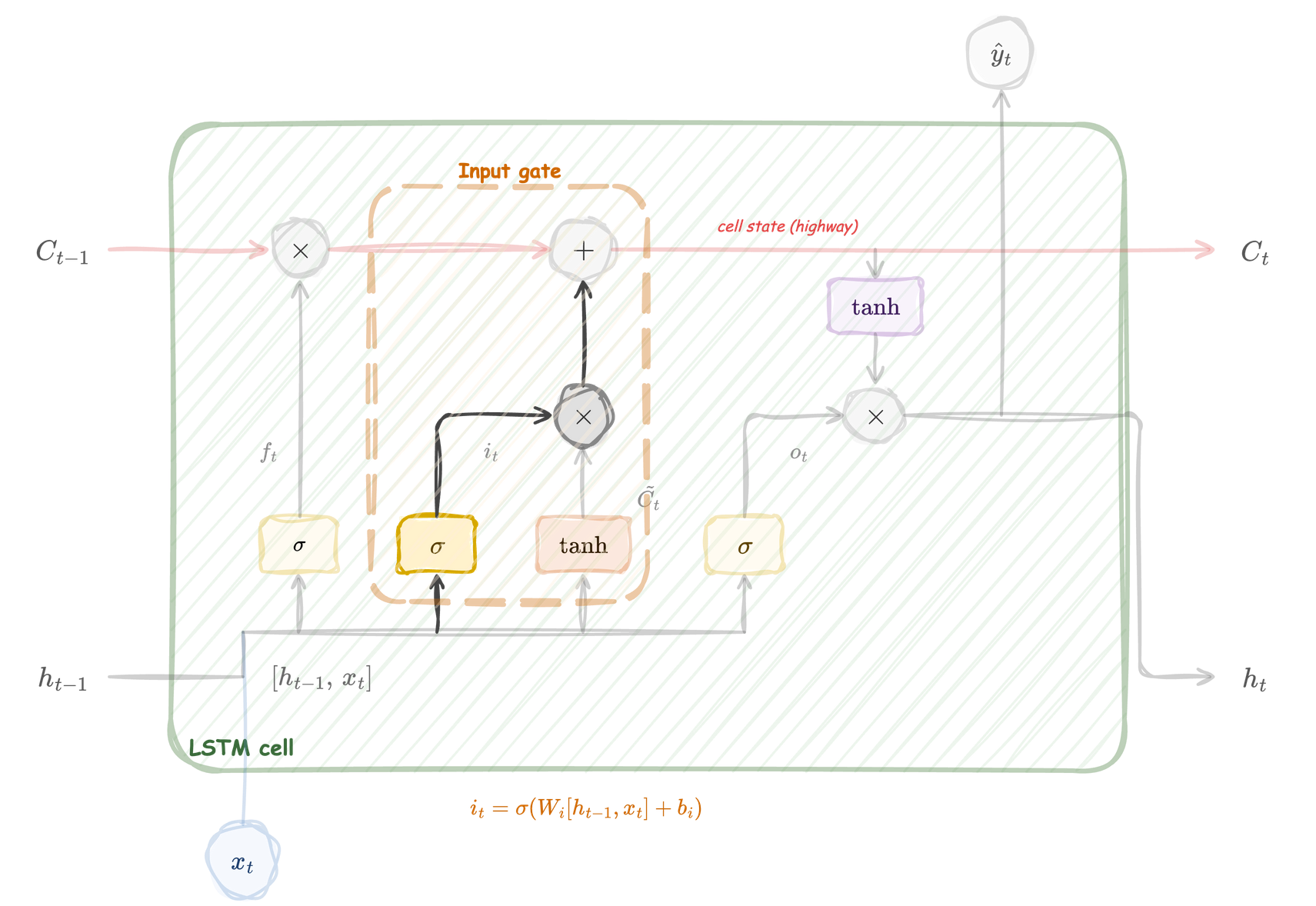
The input gate reads \([h_{t-1}, x_t]\) through a sigmoid and produces \(i_t\). It controls how much of the new candidate to write into the cell state. The input gate is the volume knob; the candidate (next) provides the content.

Input gate

\[ i_t = \sigma\!\bigl(W_i\, [h_{t-1},\, x_t] + b_i\bigr) \]

Dimensions:

• \(W_i \in \mathbb{R}^{d_h \times (d_h + d_{\text{in}})}\), \(b_i \in \mathbb{R}^{d_h}\)
• \(i_t \in (0,1)^{d_h}\): per-dimension write strength

Separation of roles:

• Input gate decides how much to write (control)
• Candidate decides what to write (content)

Draw attention to the fact that the input gate and the candidate share the same inputs but use different weight matrices and different activations. The input gate is a sigmoid (0 to 1, controlling magnitude), while the candidate is a tanh (-1 to 1, proposing signed content).

Candidate value

The candidate computes \(\tilde{C}_t\) through a \(\tanh\) activation. Unlike the three gates, it proposes content rather than control. Combined with the input gate as \(i_t \odot \tilde{C}_t\), it determines what new information enters the cell state.

Candidate value

\[ \tilde{C}_t = \tanh\!\bigl(W_C\, [h_{t-1},\, x_t] + b_C\bigr) \]

Dimensions:

• \(W_C \in \mathbb{R}^{d_h \times (d_h + d_{\text{in}})}\), \(b_C \in \mathbb{R}^{d_h}\)
• \(\tilde{C}_t \in (-1, 1)^{d_h}\): proposed content

Key properties:

• Uses \(\tanh\) (+,-)
• Only non-gate component
• Gated contribution: \(i_t \odot \tilde{C}_t\)

Point out that the candidate is structurally identical to a vanilla RNN update: a tanh applied to a linear combination of the previous hidden state and the current input. The difference is that its contribution to the cell state is gated by i_t rather than directly overwriting everything.

Cell state update

The cell state is updated by forgetting selectively and adding selectively:

\[ C_t = f_t \odot C_{t-1} + i_t \odot \tilde{C}_t \]

• \(f_t \odot C_{t-1}\): keep selected parts of the old memory
• \(i_t \odot \tilde{C}_t\): write selected parts of the new candidate
• \(\odot\) denotes element-wise (Hadamard) product

The critical difference from vanilla RNNs

This update is additive in \(C_{t-1}\). When \(f_t \approx 1\) and \(i_t \approx 0\), the cell state passes through unchanged — no matrix multiplication, no \(\tanh\) squashing. This is why gradients can survive over long distances.

This is the single most important equation in the LSTM. Write it on the board and ask: what happens if f_t = 1 and i_t = 0 for 50 consecutive steps? Answer: C_50 = C_0, perfectly preserved. No other RNN variant before the LSTM had this property.

Output gate

The output gate selects which dimensions of the squashed cell state \(\tanh(C_t)\) are exposed as \(h_t\). The cell can store information internally that it does not yet reveal — like a notebook where you choose which page to show.

Output gate

\[ o_t = \sigma\!\bigl(W_o\, [h_{t-1},\, x_t] + b_o\bigr), \qquad h_t = o_t \odot \tanh(C_t) \]

Dimensions:

• \(W_o \in \mathbb{R}^{d_h \times (d_h + d_{\text{in}})}\), \(b_o \in \mathbb{R}^{d_h}\)
• \(o_t \in (0, 1)^{d_h}\)

Two-step output:

• \(\tanh(C_t)\) \((-1, 1)\)
• \(o_t\) selects dims to reveal
• \(h_t\) feeds preds and next step

\(C_t\) can store values outside \((-1,1)\) because only the output view \(h_t\) is squashed. This gives \(C_t\) more dynamic range.

A useful analogy: the cell state is like a notebook you carry, and the output gate decides which page to show to the outside world at each step. You might store information now and reveal it only when it becomes relevant later. This is exactly how LSTMs handle tasks like bracket matching or long-range agreement.

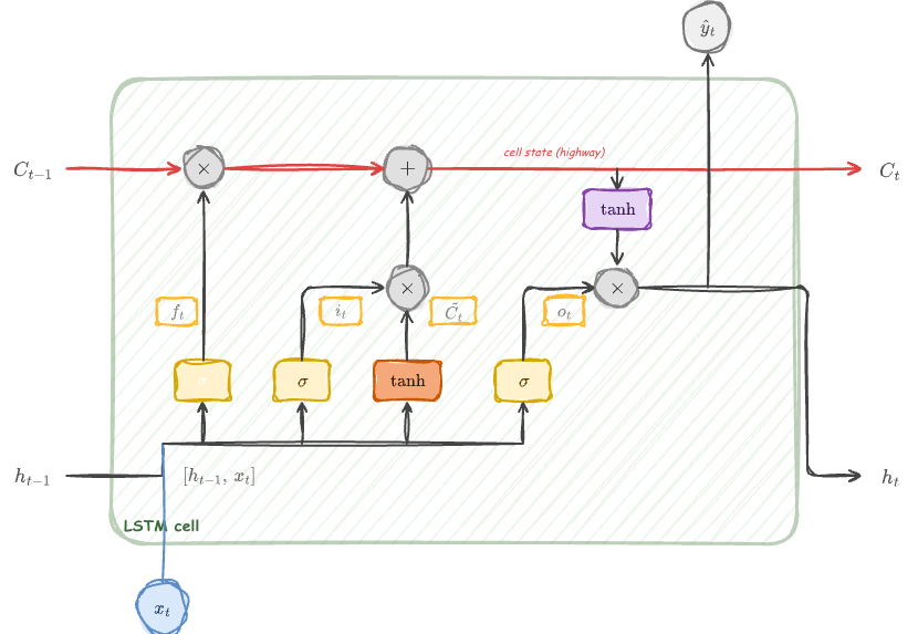
Putting it all together

Complete LSTM cell with all gates active. The red arrow shows the cell state highway; the four blocks at the bottom compute the gates and candidate from \([h_{t-1}, x_t]\).

Putting it all together

All four equations for one time step:

\[\begin{eqnarray} f_t &=& \sigma\bigl(W_f [h_{t-1}, x_t] + b_f\bigr) \\ i_t &= & \sigma\bigl(W_i [h_{t-1}, x_t] + b_i\bigr)\\ \tilde{C}_t &= & \tanh\bigl(W_C [h_{t-1}, x_t] + b_C\bigr)\\ C_t &= &f_t \odot C_{t-1} + i_t \odot \tilde{C}_t\\ o_t &= & \sigma\bigl(W_o [h_{t-1}, x_t] + b_o\bigr)\\ h_t &= & o_t \odot \tanh(C_t) \end{eqnarray}\]

Inputs: \(h_{t-1}, C_{t-1}, x_t\). Outputs: \(h_t, C_t\).

This is the summary slide. Walk through the full forward pass once more, tracing the path in the diagram: (1) forget gate filters C_{t-1}, (2) input gate and candidate add new content, (3) output gate filters C_t to produce h_t. All four weight matrices are applied in parallel in efficient implementations.

A step-by-step walkthrough

To consolidate, trace the computation for a single time step:

1. Concatenate inputs: form \([h_{t-1}, x_t] \in \mathbb{R}^{d_h + d_{\text{in}}}\)
2. Forget: compute \(f_t = \sigma(W_f [h_{t-1}, x_t] + b_f)\) — decide what to erase from memory
3. Input + Candidate: compute \(i_t\) and \(\tilde{C}_t\) — decide what new content to write
4. Update cell: \(C_t = f_t \odot C_{t-1} + i_t \odot \tilde{C}_t\) — the additive highway update
5. Output: compute \(o_t\) and \(h_t = o_t \odot \tanh(C_t)\) — decide what to expose

Tip

In practice, the four matrix multiplications (\(W_f, W_i, W_C, W_o\)) are fused into a single large multiplication and then split. This is why you will see implementations using a single weight matrix of size \(4 d_h \times (d_h + d_{\text{in}})\).

Parameter count

Each gate has its own weight matrix and bias:

• Each of the 4 weight matrices: \(W \in \mathbb{R}^{d_h \times (d_h + d_{\text{in}})}\)
• Each of the 4 bias vectors: \(b \in \mathbb{R}^{d_h}\)

Total parameters per LSTM layer:

\[ 4\, d_h\, (d_h + d_{\text{in}}) + 4\, d_h = 4\, d_h\, (d_h + d_{\text{in}} + 1) \]

Note

An LSTM has roughly 4 times the parameters of a vanilla RNN with the same \(d_h\) and \(d_{\text{in}}\). This is the cost of gating. In efficient implementations, the four matrix multiplications are fused into one large product.

Why LSTMs mitigate vanishing gradients

The LSTM cell state evolves as:

\[ C_s = f_s \odot C_{s-1} + i_s \odot \tilde{C}_s \]

where:

• \(f_s\): forget gate
• \(i_s\): input gate
• \(\tilde{C}_s\): candidate cell update

The key term is:

\[ f_s \odot C_{s-1} \]

which carries the previous memory forward by elementwise scaling.

Remember about cell state \(C_s\)

The cell state at time (s) is a vector:

\[ C_s \in \mathbb{R}^{d_h} \qquad\text{with}\qquad C_s = \begin{bmatrix} C_s^{(1)} \\ C_s^{(2)} \\ \vdots \\ C_s^{(d_h)} \end{bmatrix} \]

• \(s\) indexes the time step
• \(j\) indexes the position inside the vector
• \(C_s^{(j)}\) means the \(j\)-th component of the cell state at time \(s\)

So \(j\) simply labels one memory dimension of the LSTM.

Remember about cell state \(C_s\)

(\(j\)) is the index of one component of the hidden/cell vector, (\(s\)) is the time step. If the cell state is

\[C_s \in \mathbb{R}^{d_h}, C_s =\begin{bmatrix} C_s^{(1)}\\ C_s^{(2)}\\ \vdots\\ C_s^{(d_h)} \end{bmatrix} \]

So:

\[ C_s^{(j)} = f_s^{(j)} C_{s-1}^{(j)} + \cdots \]

Each coordinate evolves independently in that derivative, which is why the Jacobian is diagonal.

One-step gradient

Along the direct cell-state path, differentiating the cell state with respect to the previous one gives:

\[ \frac{\partial C_s}{\partial C_{s-1}} = \mathrm{diag}(f_s) \]

This is because each coordinate satisfies:

\[ C_s^{(j)} = f_s^{(j)} C_{s-1}^{(j)} + \cdots \]

so:

\[ \frac{\partial C_s^{(j)}}{\partial C_{s-1}^{(j)}} = f_s^{(j)} \]

Thus, the direct-path Jacobian is diagonal: each memory dimension is scaled independently.

Note

The full derivative also includes indirect terms because the gates depend on \(h_{s-1}\), which in turn depends on earlier states. The diagonal expression isolates the additive memory pathway that makes LSTMs trainable over longer spans.

Backpropagation through many timesteps

From time \(T\) back to time \(t\), the gradient along the cell-state path is:

\[ \frac{\partial C_T}{\partial C_t} = \prod_{s=t+1}^{T} \mathrm{diag}(f_s) \]

For each coordinate (j), this becomes:

\[ \frac{\partial C_T^{(j)}}{\partial C_t^{(j)}} = \prod_{s=t+1}^{T} f_s^{(j)} \]

So the gradient is passed backward by repeated mult. of the forget gates.

If \(f_s \approx 1\), the product stays close to 1, and gradients flow across long time spans.

Remember that \(f\) is the forget gate.

Comparing gradient paths

	Vanilla RNN	LSTM (cell state path)
Gradient factor per step	\(\mathrm{diag}(\tanh'(z_s))\; W_h\)	\(\mathrm{diag}(f_s)\)
Involves weight matrix	Yes	No
Spectral norm	Can be \(> 1\) or \(\ll 1\)	In \((0, 1)\) per element
Additive path	No	Yes
Effective memory	10–20 steps	100+ steps possible

Tip

The forget gate acts as a learnable decay rate per dimension. The network decides, based on the input, how long to retain each piece of information. This is far more flexible than the fixed decay imposed by repeated multiplication through \(W_h\).

Gradient flow: a visual comparison

Figure 11: Gradient magnitude along the cell-state path (LSTM) vs the hidden-state path (vanilla RNN)

LSTMs in bioinformatics

LSTMs have been widely applied to biological sequence tasks:

• Protein secondary structure prediction: per-residue classification over sequences of 100–1000 residues, where long-range contacts matter
• Splice site detection: dependencies between donor and acceptor sites span hundreds of nucleotides
• Clinical time series: ICU monitoring, longitudinal patient records with irregular sampling and long-term dependencies
• Gene expression forecasting: time-course experiments where early perturbations affect late responses

Note

In many of these tasks, LSTMs were the dominant architecture before Transformers. They remain a strong baseline and are often preferred when data is limited, because they have fewer parameters than attention-based models of comparable capacity.

Practical considerations

• Initialization: set forget gate biases to 1.0 so it starts by remembering
• Gradient clipping: recommended, even though LSTMs behave better than vanilla RNNs
• Stacking: multiple LSTM layers can be stacked; the output \(h_t\) of one layer becomes the input \(x_t\) of the next
• Bidirectional LSTMs: run one LSTM forward and one backward, concatenate their hidden states — useful when the full sequence is available (e.g., protein classification, but not autoregressive generation)
• Hidden size: typical values are \(d_h \in [64, 512]\) for biomedical tasks; larger values risk overfitting on small datasets

Warning

LSTMs are slower to train than vanilla RNNs (4x more parameters, 4x more computation per step) and cannot be parallelised across time steps. For very long sequences (\(T > 1000\)), consider Transformers or structured state-space models.

Gated Recurrent Unit (GRU)

Motivation: simplifying the LSTM

The LSTM introduced four components (three gates plus a candidate) and two state vectors (\(C_t\), \(h_t\)). This works well, but:

• The parameter count is 4x that of a vanilla RNN
• Two separate state vectors add implementation complexity
• For many tasks, the full gating machinery is more than necessary

The core idea

The GRU merges the cell state and hidden state into a single vector \(h_t\), and reduces the gate count from three to two: a reset gate and an update gate. It retains the key benefit of LSTMs — learnable, per-dimension control over memory retention — with fewer parameters.

Cho et al. (2014) introduced the GRU in the context of machine translation. Ask students: if the LSTM forget and input gates often move in opposite directions (forget less = write more), can we tie them together? That is exactly what the update gate does.

One state vector, two gates

A GRU cell maintains a single state vector:

• Hidden state \(h_t \in \mathbb{R}^{d_h}\) — serves as both memory and output

Two gates control how \(h_t\) is updated:

Gate	Symbol	Role
Reset	\(r_t\)	How much of \(h_{t-1}\) to use when computing the candidate
Update	\(z_t\)	How much of \(h_{t-1}\) to carry forward vs replace

Note

Compare with the LSTM: the GRU has no separate cell state \(C_t\) and no output gate. The update gate \(z_t\) plays the combined role of the LSTM forget and input gates.

The GRU cell at a glance

GRU cell: the hidden state \(h_t\) is updated through a convex combination controlled by the update gate \(z_t\). The reset gate \(r_t\) modulates how much of \(h_{t-1}\) influences the candidate \(\tilde{h}_t\).

Orient students with the full picture before diving into each gate. Point out the two sigmoid blocks (reset and update) and the tanh block (candidate). Then highlight the final interpolation step at the top.

Reset gate

The reset gate reads \([h_{t-1}, x_t]\) and produces \(r_t\) through a sigmoid. It controls how much of the previous hidden state flows into the candidate computation. When \(r_t \approx 0\), the candidate ignores the past and behaves like a plain feed-forward layer.

Reset gate

\[ r_t = \sigma\bigl(W_r\, [h_{t-1},\, x_t] + b_r\bigr) \]

Dimensions:

• \([h_{t-1}, x_t] \in \mathbb{R}^{d_h + d_{\text{in}}}\)
• \(W_r \in \mathbb{R}^{d_h \times (d_h + d_{\text{in}})}\), \(b_r \in \mathbb{R}^{d_h}\)
• \(r_t \in (0, 1)^{d_h}\)

Per-dimension behaviour:

• \(r_t^{(j)} \approx 1\): past visible to candidate
• \(r_t^{(j)} \approx 0\): past ignored by candidate

The reset gate acts only on the candidate computation, not on the final state update. It answers: when proposing new content, should we look at what we already know, or start fresh from the input alone?

Update gate

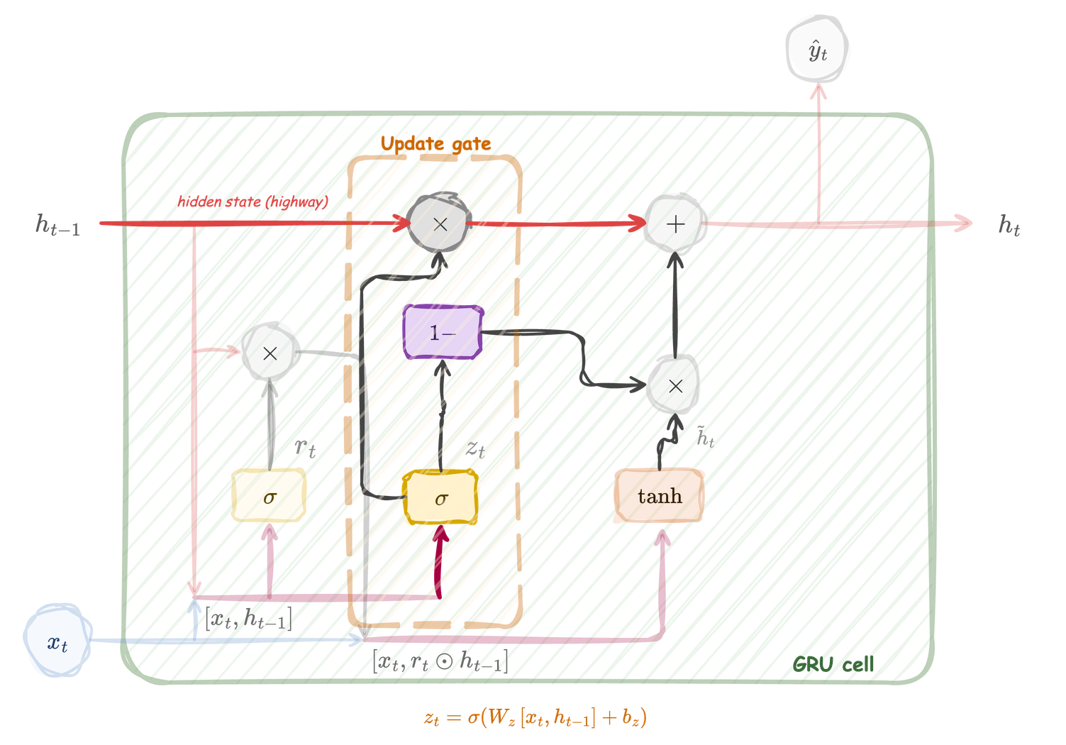
The update gate reads \([h_{t-1}, x_t]\) and produces \(z_t\) through a sigmoid. It controls the interpolation between the old state \(h_{t-1}\) and the new candidate \(\tilde{h}_t\). A value of \(z_t \approx 1\) means “keep the old state”; \(z_t \approx 0\) means “replace with the candidate”.

Update gate

\[ z_t = \sigma \bigl(W_z\, [h_{t-1},\, x_t] + b_z\bigr) \]

Dimensions:

• \(W_z \in \mathbb{R}^{d_h \times (d_h + d_{\text{in}})}\), \(b_z \in \mathbb{R}^{d_h}\)
• \(z_t \in (0, 1)^{d_h}\)

Dual role:

• \(z_t\) controls retention of \(h_{t-1}\)
• \((1 - z_t)\) controls admission of \(\tilde{h}_t\)
• One gate replaces both LSTM forget and input gates

The complementary structure \(z_t\) / \((1 - z_t)\) is what makes the GRU more parameter-efficient than the LSTM: instead of learning two independent gates that could conflict, it enforces that forgetting and writing are two sides of the same coin.

Candidate hidden state

The candidate \(\tilde{h}_t\) is computed through a \(\tanh\) activation, using the reset-gated version of \(h_{t-1}\). It proposes new content, analogous to the LSTM candidate \(\tilde{C}_t\).

Candidate hidden state

\[ \tilde{h}_t = \tanh\!\bigl(W_h\, [r_t \odot h_{t-1},\, x_t] + b_h\bigr) \]

Dimensions:

• \(W_h \in \mathbb{R}^{d_h \times (d_h + d_{\text{in}})}\), \(b_h \in \mathbb{R}^{d_h}\)
• \(\tilde{h}_t \in (-1, 1)^{d_h}\)

Key difference from LSTM:

• The reset gate modulates \(h_{t-1}\) before it enters the linear combination
• When \(r_t \approx 0\), the candidate sees only \(x_t\)

Compare with the LSTM candidate: the LSTM uses the raw h_{t-1} in the candidate computation and relies on the input gate to control writing. The GRU instead pre-filters h_{t-1} through the reset gate, giving the candidate itself the ability to decide how much history to incorporate.

Hidden state update

The new hidden state is a convex interpolation between the old state and the candidate:

\[ h_t = z_t \odot h_{t-1} + (1 - z_t) \odot \tilde{h}_t \]

• \(z_t \odot h_{t-1}\): the fraction of old memory that survives
• \((1 - z_t) \odot \tilde{h}_t\): the fraction of new content that is written
• Since \(z_t + (1 - z_t) = 1\), this is a weighted average per dimension

The additive memory mechanism

When \(z_t \approx 1\), the hidden state passes through nearly unchanged — no matrix multiplication, no \(\tanh\) compression. This is the same principle that gives LSTMs long-range gradient flow, achieved here with a simpler structure.

This is the most important equation in the GRU. Write it on the board and compare with the LSTM cell update: C_t = f_t * C_{t-1} + i_t * C_tilde. The GRU replaces two independent gates (f_t, i_t) with the complementary pair (z_t, 1 - z_t), and operates directly on h_t instead of a separate cell state.

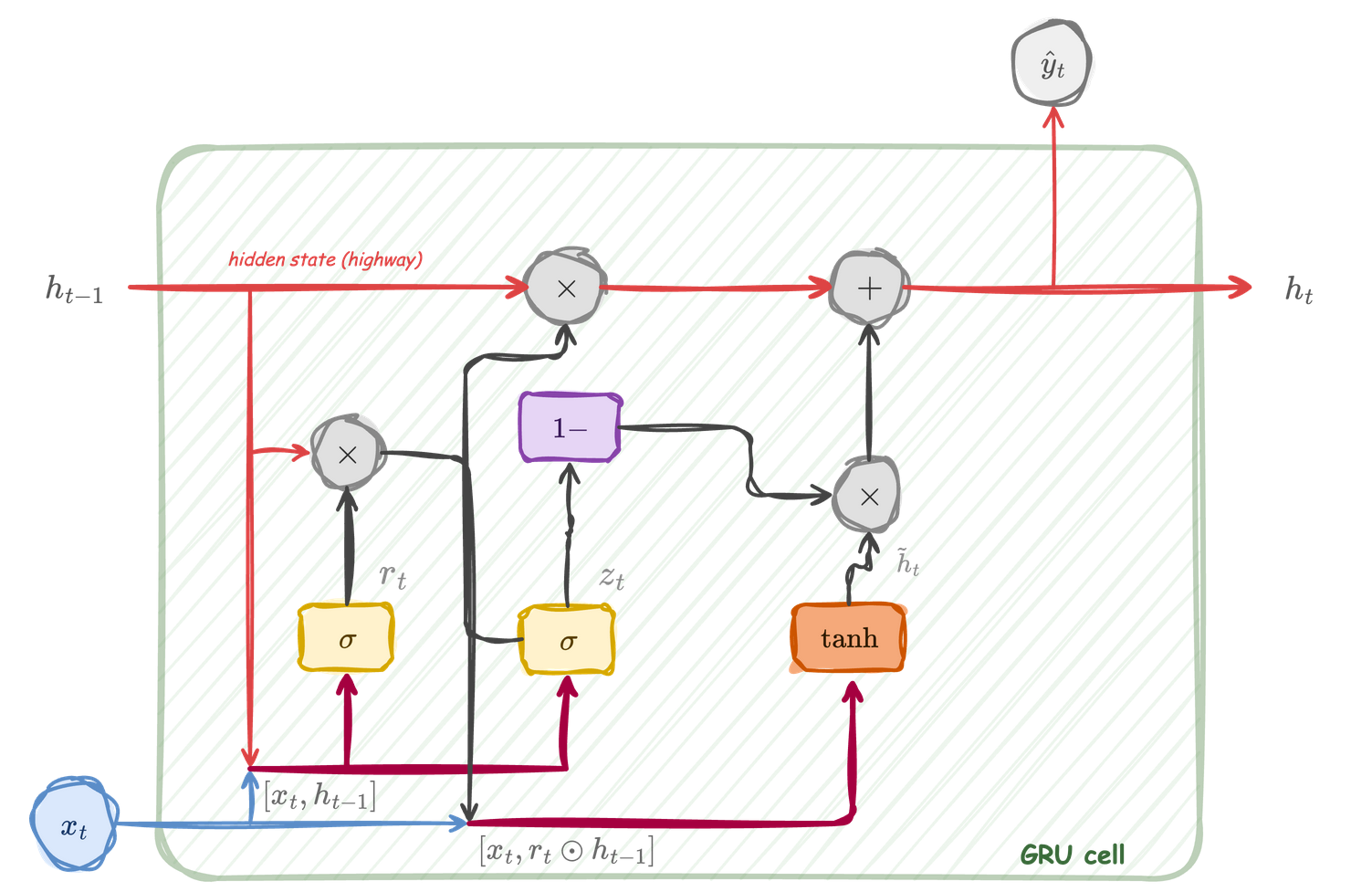
Putting it all together

Complete GRU cell. The reset gate modulates \(h_{t-1}\) for the candidate; the update gate interpolates between old and new states.

Putting it all together

All three equations for one time step:

\[\begin{eqnarray} r_t &=& \sigma\bigl(W_r [h_{t-1}, x_t] + b_r\bigr) \\ z_t &=& \sigma\bigl(W_z [h_{t-1}, x_t] + b_z\bigr) \\ \tilde{h}_t &=& \tanh\bigl(W_h [r_t \odot h_{t-1}, x_t] + b_h\bigr) \\ h_t &=& z_t \odot h_{t-1} + (1 - z_t) \odot \tilde{h}_t \end{eqnarray}\]

Input: \(h_{t-1}, x_t\). Output: \(h_t\).

Walk through the full forward pass: (1) reset gate filters h_{t-1} for the candidate, (2) update gate decides retention vs replacement, (3) candidate proposes new content using the filtered state, (4) interpolation produces h_t. All three weight matrices can be fused into a single multiplication of size 3*d_h x (d_h + d_in).

A step-by-step walkthrough

To consolidate, trace the computation for a single time step:

1. Concatenate inputs: form \([h_{t-1}, x_t] \in \mathbb{R}^{d_h + d_{\text{in}}}\)
2. Reset: compute \(r_t = \sigma(W_r [h_{t-1}, x_t] + b_r)\) — decide how much past to show the candidate
3. Candidate: compute \(\tilde{h}_t = \tanh(W_h [r_t \odot h_{t-1}, x_t] + b_h)\) — propose new content
4. Update: compute \(z_t = \sigma(W_z [h_{t-1}, x_t] + b_z)\) — decide how much to keep vs replace
5. Interpolate: \(h_t = z_t \odot h_{t-1} + (1 - z_t) \odot \tilde{h}_t\)

Tip

In practice, the three matrix multiplications (\(W_r, W_z, W_h\)) are fused into a single product using a weight matrix of size \(3 d_h \times (d_h + d_{\text{in}})\), then split and routed to the appropriate activations.

Parameter count

Each of the 3 components has its own weight matrix and bias:

• Each weight matrix: \(W \in \mathbb{R}^{d_h \times (d_h + d_{\text{in}})}\)
• Each bias vector: \(b \in \mathbb{R}^{d_h}\)

Total parameters per GRU layer:

\[ 3\, d_h\, (d_h + d_{\text{in}}) + 3\, d_h = 3\, d_h\, (d_h + d_{\text{in}} + 1) \]

Note

A GRU has 3/4 the parameters of an LSTM with the same \(d_h\) and \(d_{\text{in}}\). For the same parameter budget, a GRU can use a larger hidden size, which sometimes compensates for the simpler gating structure.

Why GRUs mitigate vanishing gradients

\[ h_t = z_t \odot h_{t-1} + (1 - z_t) \odot \tilde{h}_t \]

Differentiating with respect to the previous state (dominant term):

\[ \frac{\partial h_t}{\partial h_{t-1}} \approx \mathrm{diag}(z_t) \]

Over many steps, the gradient along the direct path is:

\[ \frac{\partial h_T^{(j)}}{\partial h_t^{(j)}} \approx \prod_{s=t+1}^{T} z_s^{(j)} \]

When \(z_s \approx 1\), the product stays close to 1 and gradients survive.

Note

This is exactly analogous to the LSTM cell-state gradient \(\prod f_s^{(j)}\), with the update gate \(z_t\) playing the role of the forget gate \(f_t\).

Comparing gradient paths: RNN vs LSTM vs GRU

	Vanilla RNN	LSTM (cell path)	GRU (hidden path)
Gradient factor	\(\mathrm{diag}(\tanh')\; W_h\)	\(\mathrm{diag}(f_s)\)	\(\mathrm{diag}(z_s)\)
Weight matrix	Yes	No	No
Additive path	No	Yes (\(C_t\))	Yes (\(h_t\))
State vectors	1 (\(h_t\))	2 (\(h_t, C_t\))	1 (\(h_t\))
Gates	0	3	2
Params (relative)	1x	4x	3x

GRU vs LSTM: when to choose which

Prefer GRU when

• Dataset is small (fewer parameters to overfit)
• Sequence lengths are moderate (\(T < 200\))
• Training speed matters (faster per step)
• A simpler model is easier to debug and interpret
• Initial baseline before scaling up

Prefer LSTM when

• Sequences are very long (\(T > 500\))
• The task requires storing information and revealing it later (output gate helps)
• You need fine-grained independent control of forgetting and writing
• Empirical results on your data favour it

Note

On many benchmarks, GRUs and LSTMs perform comparably. The choice often depends on dataset size, sequence length, and computational budget rather than on a clear architectural winner. When in doubt, try both and compare on validation data.

Chung et al. (2014) systematically compared GRU and LSTM across multiple tasks and found no consistent winner. The practical advice is: start with a GRU (simpler, faster), switch to LSTM if you see evidence that the extra gating helps on your specific problem.

GRUs in bioinformatics

GRUs have been applied to many of the same tasks as LSTMs:

• Protein function prediction: per-residue or per-sequence classification where moderate-length dependencies suffice
• Drug-target interaction: encoding molecular SMILES strings, where sequences are typically shorter than protein sequences
• Clinical event prediction: patient trajectories with tens to hundreds of time points, where the smaller parameter count reduces overfitting on limited cohorts
• Enhancer-promoter interaction: DNA sequence classification tasks where bidirectional GRUs capture local and mid-range regulatory patterns

Tip

When data is scarce — a common situation in clinical and rare-disease settings — the GRU’s lower parameter count can be a decisive advantage over the LSTM.

Secondary Structure Demo

link

Practical considerations

• Initialization: unlike the LSTM, there is no standard trick for bias initialization; default zeros work in most frameworks
• Gradient clipping: still recommended, as with any recurrent architecture
• Stacking: multiple GRU layers stack the same way as LSTMs; \(h_t\) of one layer becomes \(x_t\) of the next
• Bidirectional GRUs: same principle as bidirectional LSTMs; concatenate forward and backward \(h_t\) vectors
• Hidden size: since GRUs have 3/4 the parameters of LSTMs, you can afford a slightly larger \(d_h\) for the same compute budget

Warning

Like LSTMs, GRUs process time steps sequentially and cannot be parallelised across the time axis. For very long sequences or large-scale pretraining, Transformers are generally preferred.

Training and implementation

Why recurrent training is harder than feedforward

• In an MLP, gradients flow through a fixed, shallow graph.
• In an RNN, gradients flow through a graph unrolled \(T\) times – the effective depth equals the sequence length.
• Long sequences amplify two failure modes:
  • Vanishing gradients: signal decays exponentially with \(T\)
  • Exploding gradients: signal grows exponentially with \(T\)
• Initialisation, clipping, and gating are the main tools to keep training stable.

Note

Gates (LSTM, GRU) address vanishing gradients architecturally. The practical choices on this slide address the remaining engineering problems.

Initialisation of recurrent weights

The recurrent weight matrix \(W_h \in \mathbb{R}^{d_h \times d_h}\) is applied at every time step:

\[ h_t = \phi\bigl(W_x\, x_t + W_h\, h_{t-1} + b\bigr) \]

After \(T\) steps, the effective Jacobian involves products of \(W_h\):

\[ \frac{\partial h_T}{\partial h_0} \;\propto\; \prod_{t=1}^{T} \mathrm{diag}\bigl(\phi'(z_t)\bigr)\; W_h \]

• If \(\|W_h\| < 1\) repeatedly, gradients vanish.
• If \(\|W_h\| > 1\) repeatedly, gradients explode.

Initialisation strategies

Orthogonal initialisation (recommended default)

Sample \(W_h\) as a random orthogonal matrix: all singular values equal 1.

\[ W_h^\top W_h = I \quad\Rightarrow\quad \sigma_i(W_h) = 1 \;\;\forall\, i \]

• Preserves gradient norms at initialisation.
• Especially effective for vanilla RNNs with tanh activation.

Xavier / He for input-to-hidden

• \(W_x\): use Xavier (tanh/sigmoid) or He (ReLU), same as in feedforward layers.
• Biases: initialise to zero.

Tip

For LSTM forget gates, initialise the forget bias to 1 (or higher). This keeps the gate open at the start of training, so information flows through the cell before the network has learned what to forget.

LSTM bias initialisation in detail

Recall the LSTM forget gate:

\[ f_t = \sigma\bigl(W_f\, x_t + U_f\, h_{t-1} + b_f\bigr) \]

• At random initialisation, \(\sigma(\cdot) \approx 0.5\) on average.
• Half-open gates lose cell information from the first epoch.
• Setting \(b_f = 1\) (or \(b_f = 2\)) pushes \(f_t\) close to 1 initially.

This simple trick, proposed by Jozefowicz et al. (2015), often matters more than the choice of weight initialisation scheme.

Note

In PyTorch, nn.LSTM packs all four gate biases into one vector. You must index the correct slice to set the forget bias independently.

Gradient clipping

Even with good initialisation, occasional gradient spikes can destabilise training.

Gradient norm clipping rescales the full gradient vector when its norm exceeds a threshold \(\tau\):

\[ g \leftarrow \begin{cases} g & \text{if } \|g\| \le \tau \\[4pt] \tau \;\dfrac{g}{\|g\|} & \text{if } \|g\| > \tau \end{cases} \]

• Preserves gradient direction; only reduces magnitude.
• Typical values: \(\tau \in [1, 5]\).
• Applied after computing all gradients, before the optimiser step.

Warning

Clipping does not fix vanishing gradients. It only prevents explosions. For vanishing gradients, use gated architectures (LSTM, GRU).

Monitoring gradient norms

Logging \(\|g\|\) per training step is one of the most useful diagnostics for recurrent models.

• Healthy training: gradient norms fluctuate within a stable range (e.g., 0.1–10).
• Exploding gradients: sudden spikes to \(10^3\) or higher; training loss jumps.
• Vanishing gradients: norms collapse to \(< 10^{-4}\); loss plateaus early.

In PyTorch, compute the total norm before clipping:

total_norm = torch.nn.utils.clip_grad_norm_(
    model.parameters(), max_norm=tau
)
# total_norm is the pre-clip value -- log it

Tip

Plot gradient norms alongside the learning curve. If norms spike exactly when the loss jumps, you have an exploding-gradient event.

Monitoring hidden state saturation

For tanh or sigmoid activations, saturation means most hidden units are near \(\pm 1\) (tanh) or near 0 / 1 (sigmoid).

• Saturated units produce near-zero gradients: \(\tanh'(x) \approx 0\) for \(|x| \gg 1\).
• The network stops learning through those units.

What to check

• Histogram of \(h_t\) values across the batch at a few time steps.
• Fraction of units with \(|h_t| > 0.95\) (for tanh).
• If most units are saturated early in training, reduce the learning rate or check initialisation.

Note

LSTM cell states \(C_t\) are unbounded by design – they do not saturate. This is a key reason why LSTMs handle long-range dependencies better than vanilla RNNs.

Practical optimisation choices

Optimiser

• Adam is the standard default for recurrent models.
• Learning rate: start with \(10^{-3}\); reduce on plateau or use a scheduler.

Sequence length and batching

• Sort sequences by length; group similar lengths into batches.
• Use packed sequences (PyTorch pack_padded_sequence) to avoid computing on padding tokens.

Regularisation

• Dropout between layers, not between time steps (naive temporal dropout breaks the recurrent signal).
• Variational dropout (same mask at every step) is a principled alternative.

Practical optimisation choices (continued)

Learning rate scheduling

• ReduceLROnPlateau: halve the learning rate when validation loss stalls for \(k\) epochs.
• Cosine annealing: smooth decay; common in longer training runs.
• Warm-up (a few hundred steps at a low rate) helps if gradients are noisy at the start.

When training diverges

Symptom	Likely cause	Remedy
Loss becomes NaN	Exploding gradients	Lower \(\tau\), reduce learning rate
Loss plateaus immediately	Vanishing gradients or dead gates	Check initialisation, try LSTM/GRU
Train loss drops, val loss rises	Overfitting	Add dropout, reduce model size
Val loss is noisy	Batch too small or val set too small	Increase batch size, check data split

Worked example: sequence classification with an LSTM

Task: classify protein subcellular localisation from amino-acid sequences.

• Input: one-hot or embedding of amino acids, \(x_t \in \mathbb{R}^{d_{\text{in}}}\)
• Sequence length: variable (\(T\) ranges from tens to thousands)
• Output: one of \(k\) compartments (nucleus, cytoplasm, membrane, …)

Architecture

\[ x_t \;\xrightarrow{\text{embedding}}\; e_t \in \mathbb{R}^{d_e} \;\xrightarrow{\text{LSTM}}\; h_t \in \mathbb{R}^{d_h} \;\xrightarrow{\text{pool + linear}}\; z \in \mathbb{R}^{k} \;\xrightarrow{\text{softmax}}\; \hat{y} \]

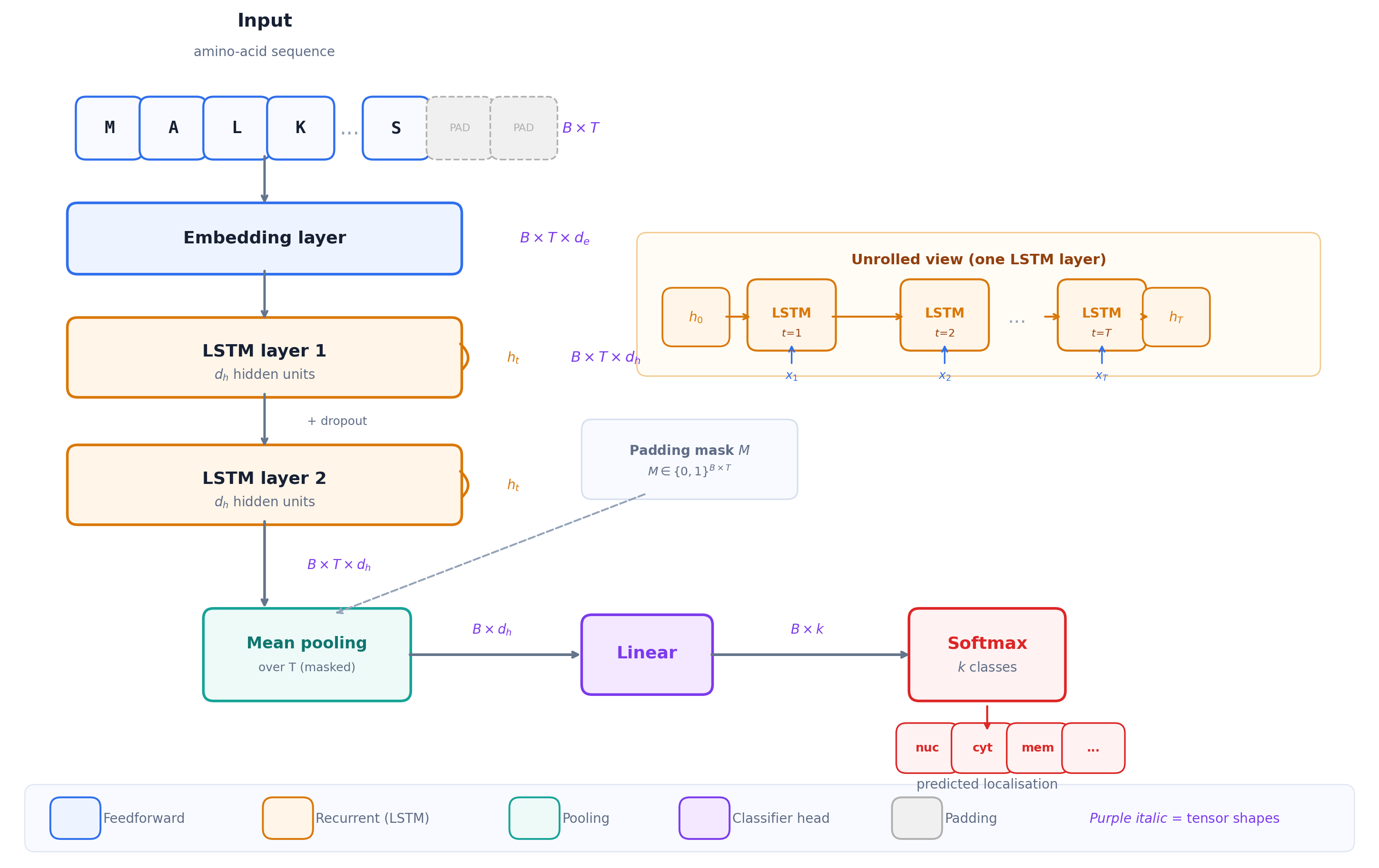
LSTM sequence classifier with embedding, recurrent layers, pooling, and softmax output

Worked example: pooling the hidden states

The LSTM produces one hidden vector \(h_t\) per time step. We need a single vector for classification.

Common pooling strategies:

• Last hidden state: \(h_T\) (simple, but biased toward the end of the sequence)
• Mean pooling: \(\bar{h} = \frac{1}{T'}\sum_{t=1}^{T'} h_t\), where \(T'\) is the true (unpadded) length
• Max pooling: \(\bar{h}_j = \max_t\, h_{t,j}\) (picks the strongest activation per dimension)

Tip

For protein sequences, mean pooling over unpadded positions is a robust default. It treats all residues equally and avoids the positional bias of using only \(h_T\).

The padding mask \(M \in \{0,1\}^{B \times T}\) is essential here: pool only over positions where \(M_{b,t} = 1\).

Worked example: training loop (pseudocode)

for epoch in 1 ... max_epochs:
    for batch in dataloader:
        x, lengths, y = batch            # padded input, true lengths, labels
        x_packed = pack(x, lengths)       # avoid computing on padding
        packed_out, _ = lstm(x_packed)    # forward pass
        h, _ = unpack(packed_out)         # padded hidden states
        pooled = masked_mean(h, lengths)  # mean over true residues
        logits = linear(pooled)           # map to k classes
        loss = cross_entropy(logits, y)

        loss.backward()                   # backward pass
        norm = clip_grad_norm_(params, tau)  # clip + log
        optimiser.step()
        optimiser.zero_grad()

    val_loss = evaluate(val_loader)
    scheduler.step(val_loss)              # reduce LR on plateau
    if val_loss < best:
        save_checkpoint()
        patience_counter = 0
    else:
        patience_counter += 1
    if patience_counter >= patience:
        break                             # early stopping

Worked example: what to monitor

During training, log at every epoch:

• Training loss and validation loss (learning curves)
• Gradient norm before clipping (stability diagnostic)
• Validation accuracy or AUROC (task-level performance)

After training, inspect:

• Confusion matrix on the held-out test set
• Per-class performance (localisation classes are often imbalanced)
• Attention to sequence length: does the model perform differently on short vs long proteins?

Warning

Split proteins by sequence identity, not by random sampling. Homologous sequences in both train and test sets inflate performance and hide poor generalisation.

Summary: training recurrent models

Concern	Recommendation
Weight init (\(W_h\))	Orthogonal; forget bias = 1 for LSTM
Gradient explosions	Clip global norm, \(\tau \in [1, 5]\)
Vanishing gradients	Use LSTM or GRU
Optimiser	Adam, lr \(\approx 10^{-3}\)
Regularisation	Dropout between layers; weight decay
Monitoring	Log gradient norms + learning curves every epoch
Stopping criterion	Early stopping on validation loss
Batching	Pack sequences; sort by length

RNN Encoder–Decoder Bridge

Why another sequence-to-sequence setting?

So far, sequence-to-sequence meant one label aligned to each input position:

\[ X = (x_1,\dots,x_T) \longrightarrow Y = (y_1,\dots,y_T) \]

Many biological and biomedical tasks are more general:

\[ X = (x_1,\dots,x_T) \longrightarrow Y = (y_1,\dots,y_{T'}) \]

where \(T'\) may differ from \(T\).

Examples:

• Translate a clinical note into structured codes
• Generate a protein sequence from a desired functional description
• Summarise a longitudinal patient trajectory into a short report
• Map one molecular representation into another sequence representation

This slide prepares the next lecture. The important point is that the output sequence is not position-aligned with the input. A per-position classifier is no longer enough; the model must read the whole source sequence, then generate a target sequence.

Encoder–decoder with RNNs

An RNN encoder reads the input sequence and compresses it into a context vector:

\[ h_t = f_{\text{enc}}(x_t, h_{t-1}), \qquad c = h_T \]

An RNN decoder generates the output sequence one token at a time:

\[ s_t = f_{\text{dec}}(y_{t-1}, s_{t-1}, c), \qquad p(y_t \mid y_{<t}, X) = \mathrm{softmax}(W_o s_t + b_o) \]

• The encoder and decoder can have different lengths: \(T \ne T'\)
• The decoder is autoregressive: each generated token conditions the next step
• During training, teacher forcing often feeds the true previous token \(y_{t-1}^\ast\)

Note

This is the classic RNN encoder–decoder idea used in neural machine translation (Sutskever et al. 2014; Cho et al. 2014).

The bottleneck problem

The encoder–decoder solves variable input/output lengths, but it creates a new problem:

\[ x_1,\dots,x_T \quad \longrightarrow \quad c = h_T \quad \longrightarrow \quad y_1,\dots,y_{T'} \]

The whole input must pass through a single fixed-size vector \(c\).

Consequences:

• Early input positions may be poorly represented in \(h_T\)
• Long sequences overload the context vector
• Gradients from decoder step \(t\) reach early encoder states only through a long recurrent chain
• Increasing \(d_h\) helps, but does not remove the sequential bottleneck

Tip

The next lecture introduces attention as the solution: instead of forcing the decoder to rely only on \(c = h_T\), let it look back at all encoder states \(h_1,\dots,h_T\) at every output step (Bahdanau et al. 2015).

Bridge to attention

RNNs gave us three ideas that Transformers keep:

• A sequence is a set of position-indexed representations
• A prediction at one position should depend on context from other positions
• Additive paths help gradients move through deep computations

Transformers change the mechanism:

Question	RNN answer	Transformer answer
How does context move?	Step by step through \(h_t\)	Directly through attention weights
How many sequential steps from position 1 to \(T\)?	\(O(T)\)	\(O(1)\) per layer
What is the bottleneck?	Fixed hidden state / context vector	Quadratic attention cost

End the RNN sessions by asking: what if every position could directly query every other position? That question is the conceptual opening of the Transformer lecture.

Notation

Notation for sequences, states, and batches

We will use the following conventions throughout the course.

Single sequence

• Input at one step: \(x_t \in \mathbb{R}^{d_{\text{in}}}\), for \(t \in \{1,\dots,T\}\)
• Full sequence as a matrix: \(X \in \mathbb{R}^{T \times d_{\text{in}}}\)
• Hidden state at step \(t\): \(h_t \in \mathbb{R}^{d_h}\)
• Cell state (LSTM only): \(C_t \in \mathbb{R}^{d_h}\)

Batch of sequences (training)

• Batch size: \(B\) (number of sequences processed together)
• Padded input tensor: \(X \in \mathbb{R}^{B \times T \times d_{\text{in}}}\), where \(T = T_{\max}\) for the batch
• Padding mask: \(M \in \{0, 1\}^{B \times T}\), where \(M_{b,t} = 0\) marks a padding position for sequence \(b\)

Tip

Sequences in a batch typically have different true lengths. Padding extends each to \(T_{\max}\) with a special token (or zeros), and \(M\) tells the model which positions to ignore in the loss and in any attention computation.

Go through each symbol and ask students to say aloud what the dimensions mean. The batch dimension \(B\) is the most commonly confused one: it stacks sequences side by side, it does not concatenate them end to end. Spend time on the mask: it appears in loss masking, in attention, and in pooling, so students will see it repeatedly.

Notation (we will reuse everywhere)

We will keep the same conventions as in the MLP slides:

• Scalars: \(b\), vectors: \(\mathbf{x}\), matrices: \(W\)
• Time index: \(t \in \{1,\dots,T\}\)
• Batch size: \(B\)

Sequence input

• Single sequence: \(x_t \in \mathbb{R}^{d_{\text{in}}}\), collected as \(X \in \mathbb{R}^{T \times d_{\text{in}}}\)
• Batch of padded sequences: \(X \in \mathbb{R}^{B \times T \times d_{\text{in}}}\)
• Optional mask: \(M \in \{0,1\}^{B \times T}\), where \(M_{b,t}=0\) means “padding”

Hidden state

• \(h_t \in \mathbb{R}^{d_h}\) (the recurrent “memory” at time \(t\))
• For gated models we will also use a cell state \(C_t \in \mathbb{R}^{d_h}\) (LSTM)

Questions

References

Anfinsen, Christian B. 1973. “Principles That Govern the Folding of Protein Chains.” Science 181: 223–30.

Bahdanau, Dzmitry, Kyunghyun Cho, and Yoshua Bengio. 2015. “Neural Machine Translation by Jointly Learning to Align and Translate.” arXiv Preprint arXiv:1409.0473.

Cho, Kyunghyun, Bart van Merriënboer, Caglar Gulcehre, et al. 2014. “Learning Phrase Representations Using RNN Encoder–Decoder for Statistical Machine Translation.” arXiv Preprint arXiv:1406.1078.

Chung, Junyoung, Caglar Gulcehre, Kyunghyun Cho, and Yoshua Bengio. 2014. “Empirical Evaluation of Gated Recurrent Neural Networks on Sequence Modeling.” arXiv Preprint arXiv:1412.3555.

ENCODE Project Consortium. 2012. “An Integrated Encyclopedia of DNA Elements in the Human Genome.” Nature 489: 57–74.

Hochreiter, Sepp, and Jürgen Schmidhuber. 1997. “Long Short-Term Memory.” Neural Computation 9 (8): 1735–80.

Hornik, Kurt, Maxwell Stinchcombe, and Halbert White. 1989. “Multilayer Feedforward Networks Are Universal Approximators.” Neural Networks 2: 359–66.

Jozefowicz, Rafal, Wojciech Zaremba, and Ilya Sutskever. 2015. “An Empirical Exploration of Recurrent Network Architectures.” Proceedings of the 32nd International Conference on Machine Learning (ICML), 2342–50.

Jumper, John et al. 2021. “Highly Accurate Protein Structure Prediction with AlphaFold.” Nature 596: 583–89.

Madani, Ali et al. 2023. “Large Language Models Generate Functional Protein Sequences Across Diverse Families.” Nature Biotechnology 41: 1099–106.

Pascanu, Razvan, Tomas Mikolov, and Yoshua Bengio. 2013. “On the Difficulty of Training Recurrent Neural Networks.” Proceedings of the 30th International Conference on Machine Learning, 1310–18.

Sutskever, Ilya, Oriol Vinyals, and Quoc V. Le. 2014. “Sequence to Sequence Learning with Neural Networks.” Advances in Neural Information Processing Systems 27.

Werbos, Paul J. 1990. “Backpropagation Through Time: What It Does and How to Do It.” Proceedings of the IEEE 78 (10): 1550–60.