Multilayer Perceptron and Learning

Advanced Topics in Machine Learning for Bioinformatics and Biomedical Engineering

Joana Gelabert

joana.gelabert.xirinachs@upc.edu

Universitat Politècnica de Catalunya - BarcelonaTech

b2slab | Institut de Recerca i Innovació en Salut (IRIS)

Dr. Alexandre Perera Lluna

Alexandre.Perera@upc.edu

Universitat Politècnica de Catalunya - BarcelonaTech

b2slab | Institut de Recerca i Innovació en Salut (IRIS)

March 9, 2026

MLPs and Backprop

Why backprop matters

Modern bioinformatics models (CNNs for sequence motifs, transformers for proteins, autoencoders for single-cell) are trained by gradient-based optimization.
Backpropagation is the efficient way to compute gradients of a loss with respect to millions of parameters.

Learning goals

Understand backprop as the chain rule on a computational graph.
Derive gradients for common layers and losses.
Implement (and debug) backprop with sanity checks.
Understand the why of activation functions.

Notation (we will reuse everywhere)

What a neuron/layer computes

A single unit (neuron) takes an input vector \(x \in \mathbb{R}^d\), computes:

Linear step (logit / pre-activation)
\[ z = w^\top x + b \]
Output (activation)
\[ a = \phi(z) \]

For a typical layer

\[ z = Wx + b,\qquad h = \phi(z) \] where

Input vector: \(x \in \mathbb{R}^{d}\)
Parameters:
- weights \(W \in \mathbb{R}^{m \times d}\), maps \((d \to m)\)
- biases \(b \in \mathbb{R}^{m}\)
Hidden layer activation: \(h \in \mathbb{R}^{m}\)
Nonlinearity: \(\sigma(\cdot)\), or \(\phi(\cdot): \mathbb{R}^{m} \to \mathbb{R}^{m}\) (applied element-wise)
Output:
- logits \(z \in \mathbb{R}^{k}\)
- predictions \(\hat{y} \in \mathbb{R}^{k}\) (e.g., probabilities after softmax; for binary, often \(\hat{y}\in(0,1))\)
Loss: \(L \in \mathbb{R}\) (a scalar)

Notation (we will reuse everywhere)

For a typical layer

\[ z = Wx + b,\qquad h = \phi(z) \] where

d: input dimensionality = number of input features. Examples: gene-expression features, k-mer counts, embedding length.
m: hidden-layer width = number of neurons (units) in the hidden layer. This is a tunable architecture choice (a hyperparameter).
k: output dimensionality = number of outputs. Examples:
- multiclass classification: \(k\) = number of classes
- regression with \(k\) targets: \(k\) = number of predicted values
- binary classification: often \(k=1\) (single logit/probability), or sometimes (k=2) if using a 2-class softmax.

The big picture

A classical neural network

The big picture

Training loop:

Forward Pass: compute predictions \(\hat{y}\) from inputs \(x\) and parameters \(\theta\).
Loss Computation: measure mismatch \(L(\hat{y}, y)\). \(L\) measures how wrong a model’s prediction is on a given example.
Backward pass (backprop): compute \(\nabla_\theta L\) efficiently.
Update: \(\theta \leftarrow \theta - \eta \nabla_\theta L\) (or Adam, etc.).

About Loss functions

What is a loss function?

A loss function measures how wrong a model’s prediction is on a given example. Given: ¡

input \(x\)
target (ground truth) \(y\)
model prediction \(\hat{y} = f_\theta(x)\)

the loss is a scalar: \[ L(\hat{y}, y) \in \mathbb{R} \]

We train the model by choosing parameters \(\theta\) that minimize the average loss over a dataset of \(n\) samples: \[ \min_{\theta}\; \frac{1}{n}\sum_{i=1}^{n} L\!\left(\hat{y}^{(i)}, y^{(i)}\right) \]

LSMS

The loss defines what good predictions mean.
Different tasks (regression, binary classification, multiclass) use different losses.

Overall loss functions

Loss functions are a big family. But in neural nets you can think of them in a few categories:

Classification losses:: Mainly

Binary: sigmoid + BCE (log loss)
Multiclass (single label): softmax + cross-entropy
Multi-label: independent sigmoid + summed BCE

Regression losses (continuous targets):: e.g., MSE, MAE, Huber, log-cosh.
Margin / ranking losses (separation or ordering):: e.g., hinge loss, triplet loss, contrastive loss.
Probabilistic / likelihood-based losses (negative log-likelihoods):: e.g., Gaussian NLL, Poisson NLL (common for count data), categorical NLL.

Overall loss functions

Distance / similarity losses (embeddings, metric learning):: e.g., cosine loss, Euclidean distance objectives.
Structured losses (sequence/structure outputs):: e.g., CTC (speech-like sequence alignment), structured SVM losses (less common in basic NN courses).
Regularization terms (often added to the loss):: e.g., ( \(\lambda|W|_2^2\) ) (weight decay), ( \(\lambda|W|_1\) ). These aren’t “prediction losses” by themselves, but they modify the objective.

In practice, use just a few core ones: MSE (regression), BCE (binary/multi-label), and softmax cross-entropy (multiclass).

Regression loss functions

Mean squared error (MSE)

Used when targets are real-valued (e.g., expression level prediction, continuous phenotype).

For a single scalar prediction \(\hat{y}\in\mathbb{R}\): \[ L_{\text{MSE}}(\hat{y},y)=\frac{1}{2}(\hat{y}-y)^2 \] (The factor \(1/2\) is convenient: it cancels in derivatives.)

Gradient w.r.t. prediction: \[ \frac{\partial L_{\text{MSE}}}{\partial \hat{y}} = \hat{y}-y \]

When it works well: Gaussian noise / squared-error is acceptable, smooth optimization.
Sensitivity: strongly penalizes outliers.

Mean absolute error (MAE)

\[ L_{\text{MAE}}(\hat{y},y)=|\hat{y}-y| \] Subgradient: \[ \frac{\partial L_{\text{MAE}}}{\partial \hat{y}} \in \mathrm{sign}(\hat{y}-y) \] (Not differentiable at \(0\); optimizers use subgradients.)

When it works well: heavier-tailed noise, robust to outliers.
Tradeoff: gradient is constant (can be slower to converge near optimum).

Huber loss (smooth robust regression)

Interpolates between MSE (near 0) and MAE (far away). For residual \(r=\hat{y}-y\) and threshold \(\delta>0\): \[ L_{\delta}(r)= \begin{cases} \frac{1}{2}r^2 & |r|\le \delta \\ \delta(|r|-\frac{1}{2}\delta) & |r|>\delta \end{cases} \] Derivative: \[ \frac{\partial L_\delta}{\partial \hat{y}}= \begin{cases} r & |r|\le \delta \\ \delta\,\mathrm{sign}(r) & |r|>\delta \end{cases} \]

The Huber loss is the convolution of the absolute value function with the rectangular function, scaled and translated. Thus it “smoothens out” the former’s corner at the origin.

Practical: often a good default when outliers exist.

MSE vs MAE vs Huber

Figure 1: Comparison of regression losses

Binary classification losses

Sigmoid + binary cross-entropy (BCE)

Logit \(z\in\mathbb{R}\), probability \(\hat{y}=\sigma(z)\in(0,1)\), label \(y\in\{0,1\}\): \[ \hat{y}=\sigma(z)=\frac{1}{1+e^{-z}} \] \[ L_{\text{BCE}}(\hat{y},y)= -\Big(y\log\hat{y} + (1-y)\log(1-\hat{y})\Big) \]

A key simplification for backprop is the derivative w.r.t. the logit¹: \[ \frac{\partial L_{\text{BCE}}}{\partial z}=\hat{y}-y \]

BCE with logits (numerically stable)

In implementations you typically avoid computing \(\log(1-\sigma(z))\) directly. A stable form is: \[ L_{\text{BCE-logits}}(z,y)=\log\big(1+e^{z}\big) - yz \] (which is equivalent to BCE after algebra).

Why it matters: prevents overflow/underflow for large \(|z|\).

BCE as a function of logit

Figure 2: Binary cross-entropy (with logits) as a function of the logit z

Multiclass classification losses

Softmax + categorical cross-entropy

Logits \(z\in\mathbb{R}^{k}\), probabilities \(\hat{y}\in\Delta^{k-1}\) ¹: \[ \hat{y}_i = \mathrm{softmax}(z)_i=\frac{e^{z_i}}{\sum_{j=1}^k e^{z_j}} \]

For one-hot \(y\in\{0,1\}^k\): \[ L_{\text{CE}}(\hat{y},y)= -\sum_{i=1}^k y_i \log(\hat{y}_i) \]

Softmax + categorical cross-entropy

Backprop simplification: \[ \frac{\partial L_{\text{CE}}}{\partial z}=\hat{y}-y \]

It is the multiclass analogue of BCE+sigmoid.

Stable computation (log-sum-exp trick)

Use: \[ \log\sum_j e^{z_j} = \alpha + \log\sum_j e^{z_j-\alpha},\quad \alpha=\max_j z_j \] to avoid overflow when some logits are large.

Cross-entropy vs margin for the correct class

Figure 3: Softmax cross-entropy decreases as the correct-class logit increases (others fixed)

Multi-label classification (independent labels)

e.g. predicting multiple functional GO annotations per protein (several labels can be 1 simultaneously).

Use \(k\) independent logits \(z\in\mathbb{R}^k\) and apply sigmoid per label: \[ \hat{y}_j = \sigma(z_j) \] Loss is a sum (or mean) of BCE across labels: \[ L=\sum_{j=1}^k \mathrm{BCE}(\hat{y}_j, y_j) \]

Gradient still has a simple per-label form: \[ \frac{\partial L}{\partial z_j} = \hat{y}_j - y_j \]

Handling class imbalance

Bioinformatics datasets often have strong imbalance (rare motifs, rare cell types, rare variants).

Weighted BCE

Let positive weight \(w_+>0\) and negative weight \(w_->0\): \[ L = -\left(w_+\,y\log\hat{y} + w_-\,(1-y)\log(1-\hat{y})\right) \] This changes the gradient scale so minority classes influence training more.

Focal loss (down-weights easy examples)

Often used for extreme imbalance. Define \(p_t=\hat{y}\) if \(y=1\), else \(p_t=1-\hat{y}\): \[ L_{\text{focal}} = -(1-p_t)^\gamma \log(p_t) \] - \(\gamma>0\) focuses learning on hard cases (where \(p_t\) is small). - Often combined with class weights.

Intuition: if an example is already confidently correct, it contributes less to the loss.

BCE vs focal loss (binary)

Figure 4: Focal loss reduces the contribution of easy positives compared to BCE

Ranking / margin-based losses (brief)

Some tasks are naturally ranking problems (e.g., scoring candidate interactions).

Hinge loss (binary, margin)

With label \(y\in\{-1,+1\}\) and score \(s\in\mathbb{R}\): \[ L_{\text{hinge}}(s,y)=\max(0, 1 - y s) \] Encourages \(ys\ge 1\) (a margin).

Often used in SVMs; less common than cross-entropy in modern deep nets, but useful conceptually.

Choosing a loss: practical guidance (bioinformatics)

Regression of continuous targets: start with MSE; switch to Huber if outliers.
Binary classification: BCE with logits (stable), consider class weights for imbalance.
Multiclass (one label per sample): softmax + cross-entropy.
Multi-label: sigmoid per label + summed BCE.
Extreme imbalance / detection-like tasks: consider focal loss (plus weights).
Uncertainty/probabilistic modeling: cross-entropy is a negative log-likelihood under a categorical model; MSE corresponds to a Gaussian likelihood (fixed variance).

Backpropagation

The big picture

If \(\theta\) is the collection of all parameters, say \(\theta = (\theta_1,\theta_2,\dots,\theta_n)\) then the gradient is the vector of partial derivatives: \(\nabla_\theta L = \left( \frac{\partial L}{\partial \theta_1}, \frac{\partial L}{\partial \theta_2}, \dots, \frac{\partial L}{\partial \theta_n} \right)\)

To train a network we will do:

Forward Pass: compute predictions \(\hat{y}\) from inputs \(x\) and parameters \(\theta\).
Loss Computation: measure mismatch \(L(\hat{y}, y)\).
Backward pass (backprop): compute \(\nabla_\theta L\) efficiently.
Update: \(\theta \leftarrow \theta - \eta \nabla_\theta L\) (or Adam, etc.). So \(\theta_j \leftarrow \theta_j - \eta \frac{\partial L}{\partial \theta_j} \quad \text{for each } j\)

link

Example single neuron with sigmoid

\[ a = w^\top x + b,\qquad \hat{y}=\sigma(a)=\frac{1}{1+e^{-a}} \]

Binary cross-entropy (BCE) for label \(y\in\{0,1\}\): \[ L(\hat{y},y) = -\left(y\log \hat{y} + (1-y)\log(1-\hat{y})\right) \]

We want gradients: \(\frac{\partial L}{\partial w}\) and \(\frac{\partial L}{\partial b}\).

Computational graph viewpoint

flowchart LR
  x((x)) --> a[$$a = w \cdot x + b$$]
  w((w)) --> a
  b((b)) --> a
  a --> yhat["$$\hat y = \sigma (a)$$"]
  yhat --> L["$$L(\hat y, y)$$"]
  y((y)) --> L

Chain rule in one line

Backprop = applying the chain rule along the edges of a graph. \[ a = w^\top x + b,\qquad \hat{y}=\sigma(a)=\frac{1}{1+e^{-a}} \]

\[ L(\hat{y},y) = -\left(y\log \hat{y} + (1-y)\log(1-\hat{y})\right) \]

If \(L\) depends on \(\hat{y}\), which depends on \(a\), which depends on \(w\):

The problem

\[ \frac{\partial L}{\partial w} = \frac{\partial L}{\partial \hat{y}} \cdot \frac{\partial \hat{y}}{\partial a} \cdot \frac{\partial a}{\partial w} \]

Backprop organizes this so we reuse intermediate derivatives.

Backpropagation

The problem

\[ \frac{\partial L}{\partial w} = \frac{\partial L}{\partial \hat{y}} \cdot \frac{\partial \hat{y}}{\partial a} \cdot \frac{\partial a}{\partial w} \]

and then

\[ w \leftarrow w - \eta \frac{\partial L}{\partial w} \]

For our example

Sigmoid: \[ \sigma'(a)=\sigma(a)\left(1-\sigma(a)\right) \]

Affine: \[ a = w^\top x + b \quad\Rightarrow\quad \frac{\partial a}{\partial w}=x,\; \frac{\partial a}{\partial b}=1 \]

Let’s derive \(\partial L/\partial a\)

Let’s derive \(\frac{\partial L}{\partial a}\)

Binary classifier (single neuron):

\[ a = w^\top x + b,\qquad \hat{y}=\sigma(a)=\frac{1}{1+e^{-a}} \]

Binary cross-entropy (BCE):

\[ L(\hat{y},y)= -\Big(y\log \hat{y} + (1-y)\log(1-\hat{y})\Big), \quad y\in\{0,1\} \]

We want the gradient w.r.t. the logit \(a\): \(\frac{\partial L}{\partial a}\).

Step 1: compute \(\frac{\partial L}{\partial \hat{y}}\)

Differentiate BCE w.r.t. \(\hat{y}\):

\[ \frac{\partial L}{\partial \hat{y}} = -\left( y\cdot \frac{1}{\hat{y}} + (1-y)\cdot \frac{-1}{1-\hat{y}} \right) = -\frac{y}{\hat{y}}+\frac{1-y}{1-\hat{y}} \]

Put over a common denominator:

\[ \frac{\partial L}{\partial \hat{y}} = \frac{-y(1-\hat{y})+(1-y)\hat{y}}{\hat{y}(1-\hat{y})} = \frac{\hat{y}-y}{\hat{y}(1-\hat{y})} \]

Step 2: compute \(\displaystyle \frac{\partial \hat{y}}{\partial a}\)

Sigmoid derivative:

\[ \hat{y}=\sigma(a)=\frac{1}{1+e^{-a}} \quad\Rightarrow\quad \frac{\partial \hat{y}}{\partial a} = \sigma(a)(1-\sigma(a)) = \hat{y}(1-\hat{y}) \]

Step 3: chain rule and the simplification

By the chain rule:

\[ \frac{\partial L}{\partial a} = \frac{\partial L}{\partial \hat{y}} \cdot \frac{\partial \hat{y}}{\partial a} \]

Substitute the two results:

\[ \frac{\partial L}{\partial a} = \left(\frac{\hat{y}-y}{\hat{y}(1-\hat{y})}\right) \cdot \left(\hat{y}(1-\hat{y})\right) = \hat{y}-y \]

The simplification !

This cancellation is why sigmoid + BCE is so clean in backprop:
the gradient at the logit is just prediction minus label!!.

For the parameters \(w,b\)

Since \(a=w^\top x + b\):

\[ \frac{\partial a}{\partial w}=x,\qquad \frac{\partial a}{\partial b}=1 \]

Therefore:

\[ \frac{\partial L}{\partial w} = \frac{\partial L}{\partial a}\frac{\partial a}{\partial w} = (\hat{y}-y)x, \qquad \frac{\partial L}{\partial b} = \hat{y}-y \]

Same pattern for softmax + cross-entropy

For multiclass logits \(z\in\mathbb{R}^k\), \(\hat{y}=\mathrm{softmax}(z)\), and one-hot \(y\):

\[ L = -\sum_{i=1}^k y_i\log(\hat{y}_i) \]

A key result (analogous to BCE+sigmoid) is:

\[ \frac{\partial L}{\partial z}=\hat{y}-y \]

So in both cases, the error signal at the final logits is \(\hat{y}-y\).

(extra) For a Vectorized setup (batch + layer view)

Batch of size \(n\):

Inputs \(X \in \mathbb{R}^{n\times d}\)
Weights \(W \in \mathbb{R}^{1\times d}\), bias \(b\in\mathbb{R}\) (binary case, one logit)
Logits \(a \in \mathbb{R}^{n\times 1}\)
Probabilities \(\hat{Y}\in(0,1)^{n\times 1}\)
Labels \(Y\in\{0,1\}^{n\times 1}\)

Layer view: \[ a = XW^\top + b \qquad \hat{Y} = \sigma(a) \]

We use the mean BCE over the batch: \[ L = \frac{1}{n}\sum_{i=1}^n \ell(\hat{y}^{(i)},y^{(i)}) \]

Binary cross-entropy per sample

For sample \(i\): \[ \ell(\hat{y}^{(i)},y^{(i)})= -\Big(y^{(i)}\log \hat{y}^{(i)} + (1-y^{(i)})\log(1-\hat{y}^{(i)})\Big) \]

Derivative wrt \(\hat{y}^{(i)}\): \[ \frac{\partial \ell}{\partial \hat{y}^{(i)}} = \frac{\hat{y}^{(i)}-y^{(i)}}{\hat{y}^{(i)}(1-\hat{y}^{(i)})} \]

Sigmoid derivative: \[ \frac{\partial \hat{y}^{(i)}}{\partial a^{(i)}}=\hat{y}^{(i)}(1-\hat{y}^{(i)}) \]

Error signal at the logits (vector form)

Chain rule per sample: \[ \frac{\partial \ell}{\partial a^{(i)}} = \frac{\partial \ell}{\partial \hat{y}^{(i)}} \cdot \frac{\partial \hat{y}^{(i)}}{\partial a^{(i)}} = \hat{y}^{(i)}-y^{(i)} \]

Stacking all samples: \[ \frac{\partial \ell}{\partial a} = \hat{Y}-Y \quad \in \mathbb{R}^{n\times 1} \]

For the mean loss: \[ \boxed{ \frac{\partial L}{\partial a} = \frac{1}{n}(\hat{Y}-Y) } \]

Note

You will often see \(\delta := \frac{\partial L}{\partial a}\) called the error signal. With mean reduction, it carries the \(\tfrac{1}{n}\) factor.

Gradients for the layer parameters \(W,b\)

Recall: \[ a = XW^\top + b \]

Using matrix calculus:

Since \(a\) depends linearly on \(W\): \[ \boxed{ \frac{\partial L}{\partial W} = \left(\frac{\partial L}{\partial a}\right)^\top X } \quad\Rightarrow\quad \frac{\partial L}{\partial W}\in\mathbb{R}^{1\times d} \]

Gradients for the layer parameters \(W,b\)

Bias gradient (sum over batch): \[ \boxed{ \frac{\partial L}{\partial b} = \sum_{i=1}^n \frac{\partial L}{\partial a^{(i)}} } \quad\Rightarrow\quad \frac{\partial L}{\partial b}\in\mathbb{R} \]

With mean loss: \[ \frac{\partial L}{\partial W}=\frac{1}{n}(\hat{Y}-Y)^\top X, \qquad \frac{\partial L}{\partial b}=\frac{1}{n}\sum_{i=1}^n(\hat{y}^{(i)}-y^{(i)}) \]

Extension: \(k\)-class softmax + cross-entropy (batch)

Now logits \(Z\in\mathbb{R}^{n\times k}\), probabilities \(\hat{Y}\in\mathbb{R}^{n\times k}\), one-hot targets \(Y\in\{0,1\}^{n\times k}\).

\[ \hat{Y}=\mathrm{softmax}(Z) \quad (\text{row-wise}) \] \[ L = -\frac{1}{n}\sum_{i=1}^n \sum_{c=1}^k Y_{ic}\log(\hat{Y}_{ic}) \]

Key result (same pattern): \[ \boxed{ \frac{\partial L}{\partial Z}=\frac{1}{n}(\hat{Y}-Y) } \]

So the last-layer error signal is still prediction minus target.

Where this plugs into an MLP

For an MLP ending in logits \(Z\):

Compute \(\hat{Y}\) (sigmoid for binary, softmax for multiclass)
Compute \(\delta^{(\text{out})} = \frac{\partial L}{\partial Z}\)

Then backprop into the previous layer: \[ \delta^{(\text{prev})} = \left(\delta^{(\text{out})}W^{(\text{out})}\right)\odot \phi'(A^{(\text{prev})}) \]

This is the standard backprop recursion.

BCE + sigmoid and the magic simplification

For BCE with sigmoid output, the gradient w.r.t. the pre-activation \(a\) is:

\[ \frac{\partial L}{\partial a} = \hat{y} - y \]

Then \[ \frac{\partial L}{\partial w} = (\hat{y}-y)\,x,\qquad \frac{\partial L}{\partial b} = (\hat{y}-y) \]

Tip

This is why logistic regression and binary classifiers are so clean to implement.

Visual intuition: derivatives of common activations

Why backprop is efficient

Naively computing each partial derivative separately is expensive.

Backprop computes all parameter gradients in time proportional to: - one forward pass + one backward pass

Roughly:

\(O(\#\text{edges in graph})\),
not \(O(\#\text{parameters} \times \#\text{operations})\).

Backprop as “messages” (reverse-mode autodiff)

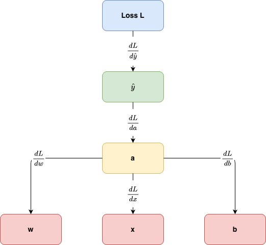
During the backward pass each node receives an upstream gradient \[ \bar{v} := \frac{\partial L}{\partial v} \] and sends downstream gradients to its parents.

What a neuron/layer computes

A single unit (neuron) takes an input vector \(x \in \mathbb{R}^d\), computes:

Linear step (logit / pre-activation)
\[ z = w^\top x + b \]
Output (activation)
\[ a = \phi(z) \]

Layer view (many neurons at once):

\[ z = Wx + b,\qquad a = \phi(z) \] where \(\phi\) is applied element-wise for most common activations.

Role of Activation Functions

Introduce non-linearity into perceptron output.
Model the behavior of biological neurons.
Examples: Step function, Sigmoid, ReLU.

Why activation functions?

A neural network layer typically computes:

\[ \mathbf{z} = \mathbf{W}\mathbf{x} + \mathbf{b}, \qquad \mathbf{a} = \phi(\mathbf{z}) \]

Without a nonlinear activation \(\phi(\cdot)\), stacking layers collapses into a single linear transformation, so the network cannot represent nonlinear relationships (crucial in bioinformatics: regulatory interactions, epistasis, nonlinear signal-response curves, etc.).

Activation functions mainly affect:

Expressivity (nonlinearity)
Optimization (gradient flow, saturation, dead units)
Output interpretation (probabilities vs real values)

Summary table

Activation	Typical use	Range	Key risk
Identity (linear)	Regression outputs	\((-\infty,\infty)\)	No nonlinearity
Sigmoid	Binary probability outputs	\((0,1)\)	Saturation, vanishing gradients
Tanh	Hidden layers (older), RNNs	\((-1,1)\)	Saturation, vanishing gradients
ReLU	Default hidden layers	\([0,\infty)\)	“Dying ReLU” (zero gradient)
Leaky ReLU	Hidden layers	\((-\infty,\infty)\)	Slope choice
ELU	Hidden layers	\((-\alpha,\infty)\)	Slightly costlier than ReLU
Softplus	Smooth ReLU alternative	\((0,\infty)\)	Still saturates for very negative inputs
GELU	Transformers / modern deep nets	\((-\infty,\infty)\)	More compute than ReLU
Softmax	Multi-class probability outputs	\((0,1)\) with sum 1	Numerical stability if naive

Identity (Linear)

\[ \phi(x) = x \]

Properties

Domain: \(\mathbb{R}\)
Range: \(\mathbb{R}\)
Differentiable everywhere; \(\phi'(x)=1\)
Monotone increasing, no saturation
Used mainly as the final layer for regression (e.g., predicting expression levels as real values)

Figure 5: Identity (linear) activation: \(\phi(x)=x\)

Sigmoid (Logistic)

\[ \sigma(x) = \frac{1}{1 + e^{-x}} \]

Properties

Domain: \(\mathbb{R}\)
Range: \((0,1)\) (interpretable as a probability)
Smooth and differentiable everywhere
Derivative: \[ \sigma'(x) = \sigma(x)\,[1-\sigma(x)] \]
Saturates for large \(|x|\) \(\Rightarrow\) vanishing gradients
Commonly used for binary classification outputs (e.g., disease vs control)

Figure 6: Sigmoid activation: \(\sigma (x)=\frac{1}{(1+e^{-x})}\)

Hyperbolic Tangent (tanh)

\[ \tanh(x) = \frac{e^x - e^{-x}}{e^x + e^{-x}} \]

Properties

Domain: \(\mathbb{R}\)
Range: \((-1,1)\) (zero-centered outputs often help optimization vs sigmoid)
Smooth and differentiable everywhere
Derivative: \[ \frac{d}{dx}\tanh(x) = 1 - \tanh^2(x) \]
Saturates for large \(|x|\) \(\Rightarrow\) vanishing gradients
Historically common in hidden layers and RNNs; now often replaced by ReLU-family activations

Figure 7: tanh activation: outputs in (-1, 1)

ReLU (Rectified Linear Unit)

\[ \mathrm{ReLU}(x) = \max(0, x) \]

Properties

Domain: \(\mathbb{R}\)
Range: \([0,\infty)\)
Piecewise linear; derivative: \[ \mathrm{ReLU}'(x)= \begin{cases} 0 & x < 0 \\ 1 & x > 0 \end{cases} \] (At \(x=0\) it is not differentiable; in practice, a subgradient is used.)
fast, encourages sparse activations, mitigates vanishing gradients on \(x>0\)
Dying ReLU — if a unit stays at \(x<0\), its gradient is 0 and it may stop learning

Leaky ReLU

\[ \phi(x)= \begin{cases} x & x\ge 0 \\ \alpha x & x<0 \end{cases} \quad \text{with } \alpha \in (0,1) \]

Properties

Domain: \(\mathbb{R}\)
Range: \(\mathbb{R}\)
Piecewise linear, not differentiable at 0 (handled with subgradients)
Derivative: \[ \phi'(x)= \begin{cases} 1 & x>0 \\ \alpha & x<0 \end{cases} \]
Reduces dying ReLU by allowing a small gradient when \(x<0\)

Figure 9: Leaky ReLU activation (\(\alpha =0.1\))

ELU (Exponential Linear Unit)

\[ \mathrm{ELU}(x)= \begin{cases} x & x\ge 0 \\ \alpha\left(e^x - 1\right) & x<0 \end{cases} \]

Properties

Domain: \(\mathbb{R}\)
Range: \((-\alpha,\infty)\)
Smooth on \(x<0\), continuous everywhere; often chosen \(\alpha=1\)
Derivative: \[ \mathrm{ELU}'(x)= \begin{cases} 1 & x>0 \\ \alpha e^x & x<0 \end{cases} \]
Negative outputs can help keep activations closer to zero mean (sometimes improving optimization)

Figure 10: ELU activation (\(\alpha =1.0\))

Softplus (Smooth ReLU)

\[ \mathrm{Softplus}(x)=\ln\left(1+e^x\right) \]

Properties

Domain: \(\mathbb{R}\)
Range: \((0,\infty)\)
Smooth approximation to ReLU
Derivative: \[ \frac{d}{dx}\mathrm{Softplus}(x)=\sigma(x) \]
For very negative \(x\), gradients become small (still some saturation), but it avoids the hard link at 0

Figure 11: Softplus activation: \(ln(1+e^x)\)

GELU (Gaussian Error Linear Unit)

A common approximation used in practice is:

\[ \mathrm{GELU}(x) \approx \frac{1}{2}x\left[1+\tanh\left(\sqrt{\frac{2}{\pi}}(x+0.044715x^3)\right)\right] \]

Properties

Domain: \(\mathbb{R}\)
Range: \(\mathbb{R}\)
Smooth, non-monotonic near the origin (it can slightly down-weight small negative inputs)
Common in Transformers and other modern architectures
More computationally expensive than ReLU/Leaky ReLU

Figure 12: GELU activation (tanh approximation)

Softmax (Multi-class output)

For logits \(\mathbf{z} \in \mathbb{R}^K\),

\[ \mathrm{Softmax}(z_i)=\frac{e^{z_i}}{\sum_{j=1}^{K} e^{z_j}} \]

Properties

Domain: \(\mathbb{R}^K\)
Range: \((0,1)^K\) with \(\sum_i p_i = 1\)
Outputs are probabilities: each in \((0,1)\) and \(\sum_i p_i = 1\)
Invariant to adding a constant: \[ \mathrm{Softmax}(\mathbf{z})=\mathrm{Softmax}(\mathbf{z}+c) \]
Needs numerical stability: compute with \(\mathbf{z}-\max(\mathbf{z})\)
Typical use: multi-class classification output layer

Figure 13: Softmax probabilities when \(z_1\) varies and \(z_2=z_3=0\) (3 classes). We vary one logit \(z_1=x\) while keeping \(z_2=z_3=0\).

All of them

Learning Curves

What is a Learning Curve?

Definition

A learning curve shows a score of an estimator for a varying number of training samples (or epochs).

Intuitively, a model should increase its learning (score) with more experience (samples or epochs).

It is common practice to plot dual curves simultaneously:

the training dataset curve, and
the validation dataset curve.

What does a Learning Curve answer?

How much does the model benefit from adding more training data?
Does the estimator suffer more from variance error or bias error?

Learning curves are heavily used when training deep neural networks, where each epoch provides a natural evaluation point.

Setup: what to track

You can configure your learning curve to maximise or minimise a score:

Maximise (higher is better): e.g., classification accuracy, F1-score, AUROC
Minimise (lower is better, target \(\approx\) 0): e.g., loss (MSE, cross-entropy, RMSE) — the most common choice in deep learning

During training, at each step you evaluate two quantities:

Train LC: Score on the training set — measures how well the model is learning.
Val LC: Score on a held-out validation set — measures how well the model is generalising.

Diagnosing Model Behaviour

What can we learn?

From the dynamics and shape of the learning curves we can diagnose:

About our model:

Underfitting
Good fitting
Overfitting

About our data:

Unrepresentative training dataset
Unrepresentative validation dataset (handle with care)

These patterns hint at issues with model capacity, dataset size, and generalisation.

Underfit — model too simple

Underfit condition

The model cannot obtain a sufficiently low error value on the training set.

Both curves plateau at a **high loss** value.

Flat curves at high loss

The model does not have sufficient capacity for the complexity of the dataset.

Causes:

Model too simple (too few parameters / layers)
Features not expressive enough
Learning rate too high

Remedy: increase model capacity, add layers, or improve features.

Underfit — training stopped too early

Underfit condition

The model cannot obtain a sufficiently low error value on the training set.

Both curves are **still decreasing** at the end of training.

Dec. Train loss · Dec. Val loss

Both curves are still falling — the model has capacity to keep improving but training was stopped prematurely.

Causes:

Too few epochs
Very aggressive early stopping criterion

Remedy: train for more epochs; revisit early-stopping patience.

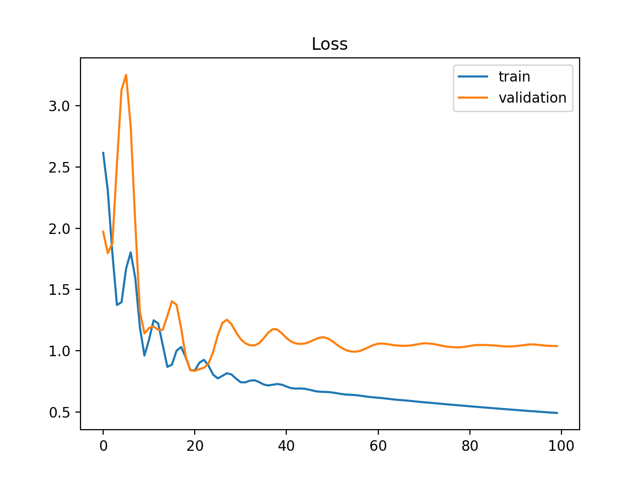
Overfit

Overfit condition

The model learns the training data too well, at the cost of increased generalisation error.

Train loss falls; val loss **rises** after the divergence point.

Dec. Train loss · Inc. Val loss

Training loss keeps decreasing while validation loss starts to increase — a clear sign the model is memorising rather than learning.

Remedies:

Regularisation (L2, dropout)
Data augmentation
Reduce model capacity
Early stopping at the divergence point

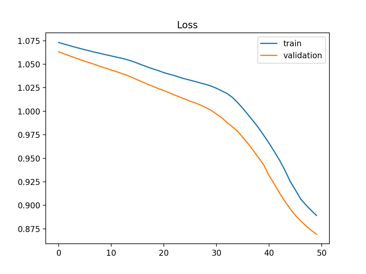
Good Fit

Good fit condition

The model learns the training data correctly and generalises well.

Both curves fall and **stabilise at a similar level**.

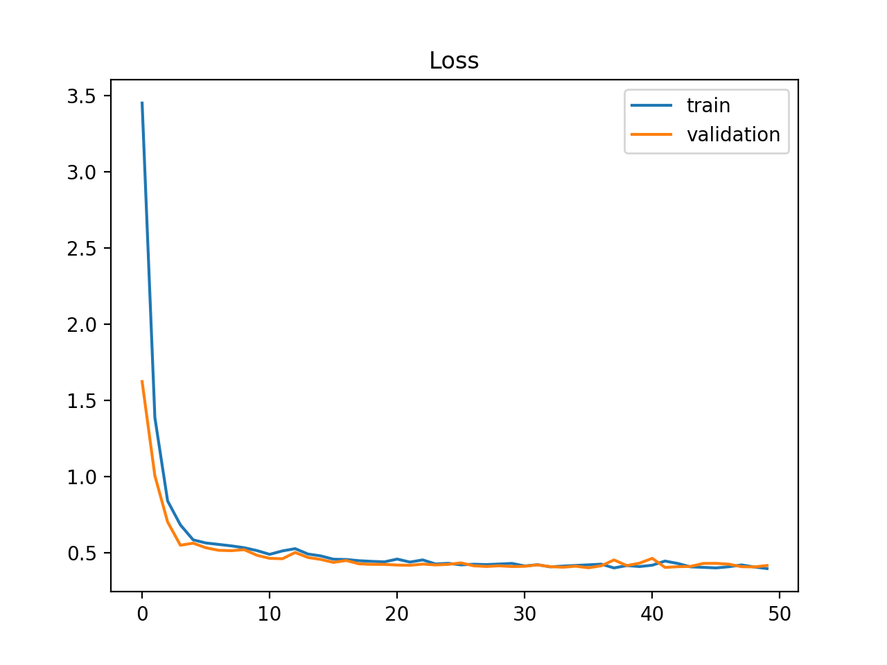
Stable Train loss · Stable Val loss

Training loss decreases and stabilises \(\checkmark\)
Validation loss follows a similar path \(\checkmark\)
Both reach a similar final value \(\checkmark\)

A small, stable gap between train and val loss is acceptable — a perfect gap of zero is unlikely in practice.

Unrepresentative Training Set

Unrepresentative training condition

The training data does not provide sufficient information to explain the validation distribution. (Sample size? Distribution shift?)

The gap between train and val loss **keeps growing**.

Dec. Train loss · Stable Val loss · Growing gap

Training loss decreases steadily
Validation loss stabilises at a much higher value
The gap between the two curves widens over time

Remedies:

Collect more training data
Apply data augmentation
Check for train/val distribution mismatch

Unrepresentative Validation Set — noisy

Unrepresentative validation condition

The validation data may not provide sufficient information to evaluate generalisation reliably.

Train loss behaves normally; val loss is **highly noisy**.

Stable Train loss · Noisy Val loss

Training loss looks like a good or acceptable fit
Validation loss shows high variance — erratic behaviour with no clear trend

Causes:

Validation set too small
Validation set not stratified / shuffled

Remedy: increase validation set size; use k-fold cross-validation.

Unrepresentative Validation Set — val below train

Unrepresentative validation condition

Validation loss systematically lower than training loss — often an artefact of the training procedure.

Val loss stays **below** train loss throughout training.

Stable Train loss · Lower Val loss · Wide gap

Training loss looks like a good fit
Validation loss converges to a value lower than training loss
The gap is persistent and wide

Common cause: dropout or other stochastic regularisation active during training but disabled during evaluation, making val loss artificially lower.

Not always a problem — understand the cause first.

Practical Notes

Why overfitting matters in bioinformatics (and everywhere)

A deep model can look brilliant on the training set and still be useless on new samples.

Think about a classifier trained to distinguish tumour subtypes from gene-expression profiles. If the network learns quirks of the training cohort rather than stable biological patterns, it will not generalise to patients from another lab, hospital, or sequencing batch.

\[ \mathcal{L}_{\text{train}} \downarrow \quad \text{while} \quad \mathcal{L}_{\text{val}} \uparrow \]

\[ \text{generalisation gap} = \mathcal{L}_{\text{val}} - \mathcal{L}_{\text{train}} \]

Note

A widening gap between training and validation loss is the classic warning sign: the model is remembering the data, not learning the signal.

Tip

In biology this is especially dangerous — datasets are often small, noisy, high-dimensional, and heterogeneous.

A healthy model improves on both sets; an overfit model keeps improving only on training data.

Recap

Dropout

About dropout

Dropout

Dropout randomly switches off neurons during training. The network cannot rely on one convenient pathway, so it learns more robust, distributed representations.

\[ \tilde{h}_i = h_i \cdot m_i, \qquad m_i \sim \mathrm{Bernoulli}(1-p) \]

At test time, dropout is disabled and activations are rescaled by \((1-p)\) to preserve expected magnitude.

Too little \((p \approx 0.1)\): barely any effect
Too much \((p > 0.7)\): optimisation becomes difficult
Typical range: 0.2–0.5 on dense layers

Tip

For omics tabular data, dropout is most effective in the fully connected layers — not at the raw input, where every feature may already be scarce.

The pattern changes every batch, forcing the network to learn redundant representations.

Weight penalties: L1 and L2 regularisation

L2 (weight decay)

\[ \mathcal{L} = \mathcal{L}_{\text{data}} + \lambda \sum_i w_i^2 \]

Large weights are penalised quadratically. The model keeps all features but with modest coefficients.

L1 (Lasso)

\[ \mathcal{L} = \mathcal{L}_{\text{data}} + \lambda \sum_i |w_i| \]

Promotes sparsity — some weights shrink to exactly zero, acting like automatic feature selection.

Warning

\(\lambda\) controls regularisation strength. Too small → no effect. Too large → underfitting. Tune it on validation data.

Tip

In transcriptomics or proteomics, L1 is attractive because sparse solutions are easier to interpret biologically.

L2 discourages extreme weights; L1 pushes many weights to exactly zero — automatic feature selection.

Batch normalisation and label smoothing

Batch normalisation

Batch norm standardises each layer’s output during training:

\[ \hat{x}_i = \frac{x_i - \mu_{\mathcal{B}}}{\sqrt{\sigma^2_{\mathcal{B}} + \varepsilon}}, \qquad y_i = \gamma \hat{x}_i + \beta \]

where \(\mu_{\mathcal{B}}, \sigma^2_{\mathcal{B}}\) are computed over the current mini-batch and \(\gamma, \beta\) are learnable. The mini-batch dependence also injects a small, healthy amount of noise.

Label smoothing

Instead of hard targets \((0, 1, 0)\), soften them slightly:

\[ y^{\text{smooth}} = (1-\alpha)\,y + \frac{\alpha}{K} \]

This reduces overconfidence and improves calibration.

Note

Label smoothing is particularly useful in biological classification tasks where labels are noisy or borderline cases exist.

Batch norm stabilises the learning signal; label smoothing prevents the model from becoming overconfident.

Early stopping and data augmentation

Early stopping

Monitor validation loss. Stop when it has not improved for \(k\) consecutive epochs (patience):

\[ \text{stop if } \mathcal{L}_{\text{val}}^{(t)} > \min_{t' < t} \mathcal{L}_{\text{val}}^{(t')} \;\text{for}\; k \text{ steps} \]

No extra parameters. Save the best checkpoint and restore it.

Data augmentation

Create extra training examples with label-preserving transforms:

Data type	Example transforms
Microscopy / histology	flip, rotate, crop, colour jitter
DNA sequences	reverse complement, masking
Protein sequences	token masking, substitutions
Expression matrices	mild noise after normalisation

Warning

Augmentation must preserve the label. A transform that changes the biology is not regularisation — it is corruption.

Early stopping controls training time; augmentation increases effective dataset diversity.

A sensible recipe in practice

Start simple

Use a model no larger than necessary. In small biological datasets, architecture size matters as much as clever regularisation.

Combine techniques

A common recipe is weight decay + early stopping, with dropout added if the dense layers are clearly overfitting.

Validate honestly

Split by patient, experiment, or batch — not by random rows. In bioinformatics, leakage hides in the structure of the data.

Practical checklist

Watch both training and validation curves throughout training.
Tune \(\lambda\), dropout rate, and patience on validation data — never on the test set.
Prefer biologically plausible augmentation strategies.
Be suspicious of near-perfect training accuracy on a small dataset.
Interpret success in terms of generalisation, not memorisation.

Note

The most important idea is not a specific trick. It is the habit of asking: “Will this model still work on new biological samples?”