Introduction

Advanced Topics in Machine Learning for Bioinformatics and Biomedical Engineering

Joana Gelabert

joana.gelabert.xirinachs@upc.edu

Universitat Politècnica de Catalunya - BarcelonaTech

b2slab | Institut de Recerca i Innovació en Salut (IRIS)

Dr. Alexandre Perera Lluna

Alexandre.Perera@upc.edu

Universitat Politècnica de Catalunya - BarcelonaTech

b2slab | Institut de Recerca i Innovació en Salut (IRIS)

February 16, 2026

Introduction

Significance of Understanding Neurons

• Understanding how biological neurons work is fundamental to neuroscience.
• Serves as inspiration for artificial neural networks in AI and machine learning.

Biological Neurons

• Biological neurons are the building blocks of the human brain and nervous system.
• They play a crucial role in processing information and enabling communication within the body:
  • Send and receive signals which allow us to move our muscles
  • Feel the external world
  • Think
  • Form memories
  • much more

Human Nervous system

In vertebrates, it consists of two main parts:

• The central nervous system (CNS).
  • Brain
  • Spinal cord
• The peripheral nervous system (PNS).
  • Mainly of nerves, connect the CNS to every other part of the body

Nervous system

Neuron Numbers

By the numbers¹:

• Human brain: 86 billion
  
• Human neocortex: ~20–23 billion
  
• Octopus: 500 million (2/3in arms)
  
• Honey bee: 950,000
  
• Aplysia: 18,000–20,000
  
• Leech ganglion: 350
  
• Human spinal cord: 1 billion

Aplysia is a genus of medium-sized to extremely large sea slugs

1. From Eric H. Chudler, U. Washington

Neuron Types in Spinal Cord

from iStockphoto and Queensland Brain Institute

Myelin is a lipid-rich material that in most vertebrates surrounds the axons of neurons to insulate them and increase the rate at which electrical impulses (called action potentials) pass along the axon.

Motor Neurons

Also known as efferent neurons.

• Located in the motor cortex, brainstem or the spinal cord. Spinal motor neurons may have a 1m length
• Role: Connect the spinal cord (CNS) to muscles, glands, and organs.
  
• Function: Transmit impulses to skeletal and smooth muscles -> control all voluntary & involuntary movements.
  • Upper motor neurons: Brain -> spinal cord
    
  • Lower motor neurons: Spinal cord -> muscle
• Structure: Multipolar neurons with one axon and several dendrites — the most common nerve cell body.

Smooth muscle is found in the walls of hollow organs, including the stomach, intestines, bladder and uterus. In the walls of blood vessels, and lymph vessels, (excluding blood and lymph capillaries) it is known as vascular smooth muscle.

Sensory Neurons

Also known as afferent neurons

• Convert a specific type of stimulus, via their receptors, into action potentials or graded receptor potentials.

• Role: Activated by sensory input from the environment.
  

• Types of input:

  • Physical: sound, touch, heat, light
    
  • Chemical: taste, smell
    

• Structure: Mostly pseudounipolar — one axon split into two branches.

Interneurons

Also called internuncial neurons

• And also called association neurons, connector neurons, or intermediate neurons
• Role: Link sensory neurons and motor neurons within the CNS.
  
• Functions:
  • Relay signals between sensory and motor neurons
    
  • Communicate with each other -> form complex neural circuits
    
• Structure: Multipolar, like motor neurons.

Brain Neurons: A Complex Story

• In the spinal cord, neuron types are easy to classify (sensory, motor, interneurons).
  
• In the brain, neuron diversity is enormous – tens to hundreds of types within one region.
  
• Classification challenges:
  • Different shapes, sizes, genes, electrical properties
    
  • Varying inputs, outputs, and projection patterns
    
  • Even neurons using the same neurotransmitter (e.g., GABA) can target different parts of other neurons.
• So no universal classification yet – ongoing research into the brain’s vast neuronal diversity.

Structure and Components of a Neuron

Dendrites

Receive incoming signals from other neurons.

Cell Body (Soma)

Contains the nucleus and processes signals.

Axon

Transmits signals away from the neuron.

Axon Terminal

Communicates with other neurons or cells.

Communication and Components of a Neuron

Neuron at Rest

• Neurons maintain a resting membrane potential.
• Ion channels regulate the flow of ions, maintaining an electrical gradient.

Action Potential

• When a stimulus is strong enough, an action potential is generated.
• It is an all-or-nothing electrical signal that travels down the axon.

Synaptic Transmission

• Action potentials reach the axon terminals.
• Neurotransmitters are released into the synaptic cleft.
• Neurotransmitters bind to receptors on the dendrites of the next neuron.

s The synaptic cleft is a junction or small gap at which neurons communicate with each other.

Synapse

Action Potential

Action Potential

Neurotransmission

Neurotransmission

A Bit About Neuron Models

Simplest Model

• \(x_1, x_2, \dots, x_n\) signals from other neurons or sensors (Gerstner et al. 2014)¹.
• Input weight \(w_i\), representing its strength or importance.
• The neuron sums inputs, adds a bias \(b\), then applies a activation \(H(\cdot)\).

\[ y = H\left( \sum_{i=1}^{n} w_i x_i + b \right) \]

• \(H(z) = 1\) \(\begin{cases} 1, & z \geq 0 \\ 0, & z < 0 \end{cases}\) (Heaviside step function)
• \(y\) is the output \(y \in \{0,1\}\)

1. https://neuronaldynamics.epfl.ch/book.html

Simplest Model

Weighted sum

equivalent to summing excitation/inhibition in dendrites.

Threshold

mimics “all-or-none” firing decision.

Limitations

• Ignores time — no dynamics or temporal integration.
• Ignores spikes — outputs are binary, not spike trains.
• No adaptation or synaptic plasticity.

Simple Integrate-and-Fire

• Treats the neuron as a capacitor that integrates incoming current over time, when \(V(t) \geq V_{th}\), the neuron emits a spike and \(V(t)\) is reset
• Captures the all-or-none nature of spikes, but ignores spike shape

\[ \tau_m \frac{dV}{dt} = R \cdot I(t) \]

• \(\tau_m\) = membrane time constant, \(R\) = membrane resistance (typ. in M\(\Omega\))
  • Large \(\tau_m\) → slow changes, more “memory” of past input
  • Small \(\tau_m\) → rapid changes, less integration of past input
• \(I(t)\) = input current (typ. in nA), represents the sum of all incoming synaptic currents.
• \(V(t)\) without any input (\(I(t) = 0\)), the potential decays toward 0 in this simplified form.

Leaky Integrate-and-Fire

• Treats the neuron as a capacitor that integrates incoming current over time, when \(V(t) \geq V_{th}\), the neuron emits a spike and \(V(t)\) is reset
• Captures the all-or-none nature of spikes, but ignores spike shape

\[ \tau_m \frac{dV}{dt} = -(V(t) - V_{rest}) + R \cdot I(t) \]

• Adds a “leak” term to model passive loss of charge across the membrane
  
• Voltage decays toward a resting potential \(V_{rest}\) in absence of input
  
• Still fires when \(V(t) \geq V_{th}\), then resets
  
• Can include refractory period where neuron is unable to fire- \(V_{rest}\) = resting membrane potential
  
• \(R\) and \(\tau_m\) as before

Integrate-and-Fire

Leaky Integrate-and-Fire

Adaptive Integrate-and-Fire Model

• Captures more realistic neuronal firing patterns seen in biology.
• Incorporates an adaptation variable that modulates firing threshold or membrane potential.

1. Membrane potential integrates incoming current.
2. When it crosses threshold, a spike is emitted.
3. Threshold or adaptation current is adjusted to make subsequent spikes harder for a short period.

Adaptive Integrate-and-Fire — Equations

\[ C \frac{dV}{dt} = -g_L (V - E_L) + I(t) - w \]

\[ \tau_w \frac{dw}{dt} = a (V - E_L) - w \]

Spike condition:

• If \(V \geq V_{th}\):
  • Emit spike
  • \(V \to V_{reset}\)
  • \(w \to w + b\)

Parameters:

• \(C\): Membrane capacitance
  
• \(g_L\): Leak conductance
  
• \(E_L\) Resting potential
  
• \(a, b\): Adaptation strength
  
• \(\tau_w\): Adaptation time constant

Adaptive Integrate and Fire (ADIF)

Spike-Timing Dependent Plasticity (STDP)

• STDP updates a synaptic weight \(w\) based on spike timing.

• Let the timing difference be: \[\Delta t = t_{post} - t_{pre}\]

• \(t_{pre}\) = the time when the presynaptic neuron (the neuron sending the signal along the synapse) fires a spike.

• \(t_{post}\) = the time when the postsynaptic neuron (the neuron receiving the signal) fires a spike.

Spike-Timing Dependent Plasticity (STDP)

• Updates a synaptic weight based on spike timing.

• Let the timing difference be: \[\Delta t = t_{post} - t_{pre}\]

  • If the presynaptic spike happens shortly before the postsynaptic spike, then \(\Delta t > 0\) and the synapse is potentiated (weight increases).
  • If the postsynaptic spike happens first, then \(\Delta t < 0\) and the synapse is depressed (weight decreases).

• The closer the spikes occur in time, the larger the change in weight.

Spike-Timing Dependent Plasticity (STDP)

• Learning depends on precise spike timing.

\[ \Delta w = \begin{cases} A_+ e^{-\Delta t / \tau_+}, & \Delta t > 0 \\ -A_- e^{\Delta t / \tau_-}, & \Delta t < 0 \end{cases} \]

• Potentiation (pre before post, \(\Delta t>0\)): \[\Delta w = A_{+}\exp\left(-\frac{\Delta t}{\tau_{+}}\right)\]
• Depression (post before pre, anticausal \(\Delta t<0\)): \[\Delta w = -A_{-}\exp\left(\frac{\Delta t}{\tau_{-}}\right)\]

Beyond basic STDP: extra learning mechanisms

• Weight dependence (multiplicative STDP)
  The update depends on the current synaptic strength \(w\), e.g.: \[\Delta w = f(\Delta t)\,g(w)\]

• Homeostatic scaling (stabilize activity)
  If \(w\) too much/too little, \(w\) are scaled to push toward a target rate \(r^{*}\): \[w_i \leftarrow w_i\left(1+\eta\,(r^{*}-r)\right)\] where \(r\) is the current firing rate and \(\eta\) is a small step size.

• Metaplasticity (plasticity of plasticity)
  The ability to learn changes over time: parameters like learning rate or thresholds adapt based on activity/history, e.g.: \[A_{+}=A_{+}(r), \qquad A_{-}=A_{-}(r)\]

Neuron Learning

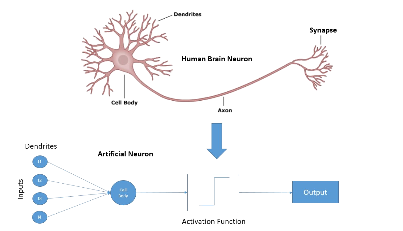
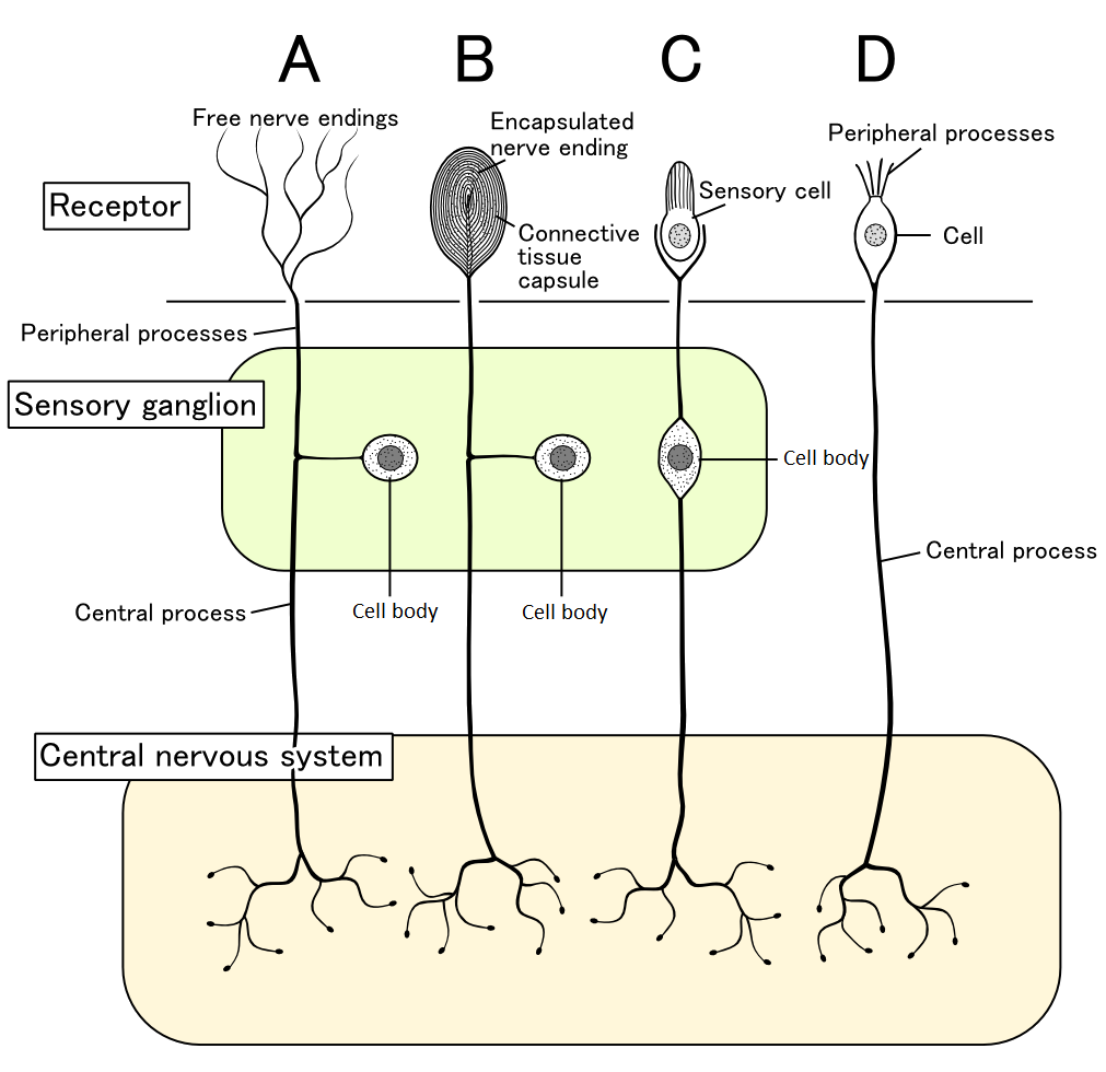
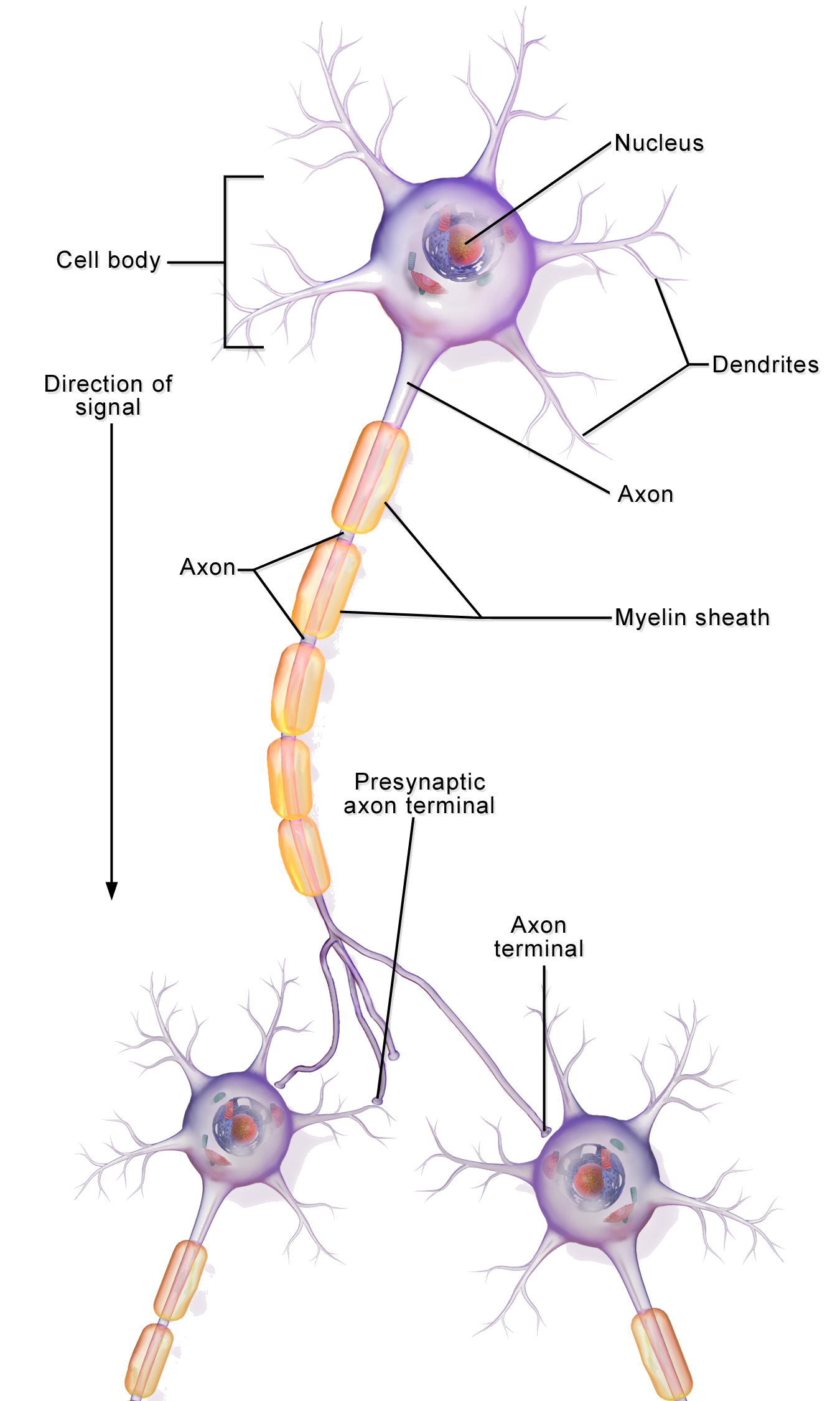
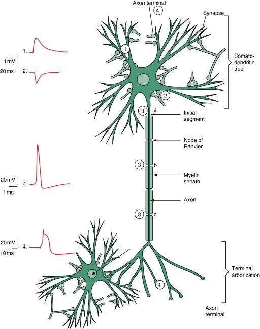
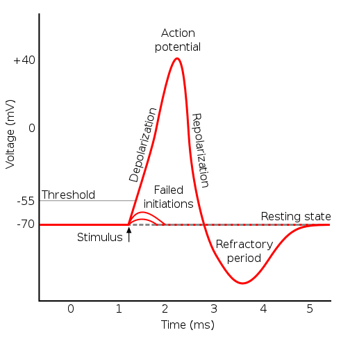
Biological Motivation

• Neurons communicate via action potentials (spikes).
  
• Learning corresponds to changes in synaptic weights.

Hebbian Learning

• Hebb postulate, from Empirical findings (Donald Hebb, 1949):

  “When an axon of cell A is near enough to excite cell B and repeatedly or persistently takes part in firing it, some growth process or metabolic change takes place in one or both cells such that A ’s efficiency, as one of the cells firing B , is increased”

• Also:

  “Cells that fire together, wire together.”

Donald Olding Hebb

Hebbian Learning

Assume a simple model of a neuron \(j\), represented as

\[ y_j = \mathbf{w_j}^\top \mathbf{x} \]

\[ \Delta w_{ij} = \eta y_j x_i \]

\[ \Delta \mathbf{w_{j}} = \eta \, ( \mathbf{w_j}^\top \mathbf{x} ) \mathbf{x} \]

If we use a set of data patterns for learning \(\mathbf{S}\): \[ \Delta \mathbf{w_{j}} = \sum_s ( \mathbf{w_j}^\top \mathbf{x^s} ) \mathbf{x^s} \equiv \eta \langle ( \mathbf{w_j}^\top \mathbf{x} ) \mathbf{x} \rangle_S \]

Hebbian Learning

• Weight update proportional to pre- and post-synaptic activity:

\[ \Delta w_{ij} = \eta \, x_i \, y_j \]

• \(x_i\) : presynaptic activity
  

• \(y_j\) : postsynaptic activity
  

• \(\eta\): learning rate

• Vector form for one postsynaptic unit with input vector \(\mathbf{x}\) and output \(y\):

\[ \Delta \mathbf{w} = \eta \, y \, \mathbf{x} \]

• Problem is that weights grow without bound.

Hebbian Learning

\[ \Delta \mathbf{w_{j}} = \eta \langle ( \mathbf{w_j}^\top \mathbf{x} ) \mathbf{x} \rangle_S \]

Hebbian Learning

\[ \Delta \mathbf{w_{j}} = \eta \langle ( \mathbf{w_j}^\top \mathbf{x} ) \mathbf{x} \rangle_S \]

Hebbian Learning

\[ \Delta \mathbf{w_{j}} = \eta \langle ( \mathbf{w_j}^\top \mathbf{x} ) \mathbf{x} \rangle_S \]

Hebbian Learning

\[ \Delta \mathbf{w_{j}} = \eta \langle ( \mathbf{w_j}^\top \mathbf{x} ) \mathbf{x} \rangle_S \]

Hebb II — Consequences and Normalization

• Correlation seeking: weights align with input directions that co-vary with \(y\).
  
• Unbounded growth without constraints:

\[ \lVert \mathbf{w}_{t+1} \rVert^2 = \lVert \mathbf{w}_t \rVert^2 + 2\eta\, y\, \mathbf{w}_t^\top \mathbf{x} + \eta^2 y^2 \lVert \mathbf{x} \rVert^2 \]

• Practical stabilizations:
  • Weight clipping: \(w_{ij} \leftarrow \mathrm{clip}(w_{ij}, w_{\min}, w_{\max})\)
  • Weight decay: \(\Delta w_{ij} = \eta \, x_i \, y_j - \lambda w_{ij}\)
  • Post-update normalization: \(\mathbf{w} \leftarrow \mathbf{w}/\lVert \mathbf{w} \rVert\)
  • Oja’s modification (for comparison): \(\Delta w_{ij} = \eta \, y \, (x_i - y \, w_{ij})\)

Oja’s Rule

• Modification of Hebbian rule with normalization:

\[ \Delta w_{ij} = \eta \, y_j \, (x_i - y_j w_{ij}) \]

• Prevents weight divergence.

Oja’s Rule I: normalization effect

• Original Oja correction

\[ \Delta w_{i} = \eta \, y \, (x_i - y w_{i}) \]

• For the case \(\qquad (y \ll 1)\)

\[ \Delta w_{i} = \eta \, y \, \bigl(x_i - \cancel{y w_{i}}\bigr) = \eta y x_i \]

• For the case \(\qquad (y \gg 1)\)

\[ \Delta w_{i} = \eta \, y \, \bigl(\cancel{x_i} - y w_{i}\bigr) = - \eta y^2 w_i \]

Stability analysis for Oja’s correction

\[ y = \mathbf{w}^\top \mathbf{x} \]

\[ \eta^{-1} \Delta \mathbf{w} = y \mathbf{x} - y^2 \mathbf{w} \]

We can evaluate three aspects of the Oja correction:

1. How do the weights evolve as we train ?
2. Which are the stationary values of the weights ?
3. Which weights vectors are stable ?

How do the weights evolve as we train ?

Let’s simplify a bit the update rule

\[ \begin{eqnarray} \eta^{-1} \Delta \mathbf{w} &=& \langle y \mathbf{x} - y^2 \mathbf{w} \rangle \\ &=& \langle ( \mathbf{w}^\top \mathbf{x}) \mathbf{x} - ( \mathbf{w}^\top \mathbf{x})^2 \mathbf{w} \rangle \\ &=& \langle \mathbf{x} ( \mathbf{w}^\top \mathbf{x}) - ( \mathbf{w}^\top \mathbf{x}) ( \mathbf{w}^\top \mathbf{x}) \mathbf{w} \rangle \\ &=& \langle \mathbf{x} ( \mathbf{x}^\top \mathbf{w}) - ( \mathbf{w}^\top \mathbf{x}) ( \mathbf{x}^\top \mathbf{w}) \mathbf{w} \rangle \\ &=& \langle ( \mathbf{x} \mathbf{x}^\top ) \mathbf{w} - ( \mathbf{w}^\top ( \mathbf{x} \mathbf{x}^\top ) \mathbf{w}) \mathbf{w} \rangle \\ &=& \langle \mathbf{x} \mathbf{x}^\top \rangle \mathbf{w} - ( \mathbf{w}^\top \langle \mathbf{x} \mathbf{x}^\top \rangle \mathbf{w}) \mathbf{w} \\ &=& C \mathbf{w} - ( \mathbf{w}^\top C \mathbf{w}) \mathbf{w} \\ \end{eqnarray} \]

So

\[ \eta^{-1} \Delta \mathbf{w} = (C-\mathbf{w}^\top C \mathbf{w} ) \mathbf{w} \]

Which are the stationary values of the weights ?

Given by \[ \eta^{-1} \Delta \mathbf{w} = 0 \] So \[ C\mathbf{w} = (\mathbf{w}^\top C \mathbf{w} ) \mathbf{w} \] if we define \(\lambda = \mathbf{w}^\top C \mathbf{w}\) we retreive a standard eigenvalues problem: \[ C\mathbf{w} = \lambda \mathbf{w} \] in which we see that
\[ \lambda = \mathbf{w}^\top C \mathbf{w} = \mathbf{w}^\top \lambda \mathbf{w} = \lambda ||\mathbf{w} ||^2 \]

So in stationary case the norm of \(\mathbf{w}\) must be 1.

Which are the stationary values of the weights ?

In summary, in stationary values of the weights \(\eta^{-1} \langle \Delta \mathbf{w} = 0 \rangle\):

• In stationary case the norm of \(\mathbf{w}\) must be 1 .
• \(C\mathbf{c_k} = \lambda_k \mathbf{c_k}\)

Which weights vectors are stable ?

We have this dynamics: \[ \eta^{-1} \Delta \mathbf{w} = C\mathbf{w} - (\mathbf{w}^\top C \mathbf{w} ) \mathbf{w} \]

Then, we can perturbate \(\mathbf{w}\) around \(e_\alpha\) to see its dynamics stability points:

\[ \mathbf{w} = e_\alpha + \varepsilon \]

Substitute into \(\eta^{-1} \Delta \mathbf{w}\)

Which weights vectors are stable I?

Substitute into \(\eta^{-1} \Delta \mathbf{w}\), you will find¹: \[ \begin{aligned} \eta^{-1}\Delta \mathbf{w} &= C(e_\alpha+\varepsilon) -\bigl((e_\alpha+\varepsilon)^\top C(e_\alpha+\varepsilon)\bigr)(e_\alpha+\varepsilon) \\ &= (Ce_\alpha + C\varepsilon) -\Bigl(e_\alpha^\top C e_\alpha + e_\alpha^\top C\varepsilon + \varepsilon^\top C e_\alpha + \varepsilon^\top C\varepsilon\Bigr)(e_\alpha+\varepsilon) \\ &= Ce_\alpha + C\varepsilon -(e_\alpha^\top C e_\alpha)e_\alpha -(e_\alpha^\top C e_\alpha)\varepsilon -(e_\alpha^\top C\varepsilon)e_\alpha -(\varepsilon^\top C e_\alpha)e_\alpha + \mathcal{O}(\|\varepsilon\|^2) \\ &= \lambda_\alpha e_\alpha + C\varepsilon -\lambda_\alpha e_\alpha -\lambda_\alpha \varepsilon -(e_\alpha^\top C\varepsilon)e_\alpha -(\varepsilon^\top C e_\alpha)e_\alpha + \mathcal{O}(\|\varepsilon\|^2) \\ &= (C-\lambda_\alpha I)\varepsilon -\Bigl(e_\alpha^\top C\varepsilon+\varepsilon^\top C e_\alpha\Bigr)e_\alpha + \mathcal{O}(\|\varepsilon\|^2) \\ &= (C-\lambda_\alpha I)\varepsilon -2\lambda_\alpha (e_\alpha^\top \varepsilon)\,e_\alpha + \mathcal{O}(\|\varepsilon\|^2), \end{aligned} \]

1. \(\begin{aligned} C e_\alpha &= \lambda_\alpha e_\alpha \\ e_\alpha^\top C^\top &= \lambda_\alpha e_\alpha^\top\\ e_\alpha^\top C &= \lambda_\alpha e_\alpha^\top \end{aligned}\)

Which weights vectors are stable ?

So

\[ \eta^{-1}\Delta \mathbf{w} = (C-\lambda_\alpha I)\varepsilon -2\lambda_\alpha (e_\alpha^\top \varepsilon)\,e_\alpha + \mathcal{O}(\|\varepsilon\|^2) \]

Which weights vectors are stable I?

We can simplify by projecting againt one eigenvector \(e_\beta\); \[ \begin{aligned} \eta^{-1} e_\beta^\top \Delta \varepsilon &\approx e_\beta^\top\Bigl[(C-\lambda_\alpha I)\varepsilon -2\lambda_\alpha (e_\alpha^\top \varepsilon)\,e_\alpha\Bigr] \\[4pt] &= e_\beta^\top C\varepsilon -\lambda_\alpha e_\beta^\top \varepsilon -2\lambda_\alpha (e_\alpha^\top \varepsilon)\, e_\beta^\top e_\alpha \\[4pt] &= \lambda_\beta e_\beta^\top \varepsilon -\lambda_\alpha e_\beta^\top \varepsilon -2\lambda_\alpha (e_\alpha^\top \varepsilon)\,\delta_{\alpha\beta} \\[4pt] &= (\lambda_\beta-\lambda_\alpha)\,e_\beta^\top \varepsilon -2\lambda_\alpha \delta_{\alpha\beta}\, e_\alpha^\top \varepsilon \\[8pt] &= \begin{cases} -2\lambda_\alpha\, e_\alpha^\top \varepsilon, & \beta=\alpha,\\[4pt] (\lambda_\beta-\lambda_\alpha)\, e_\beta^\top \varepsilon, & \beta\neq \alpha. \end{cases} \end{aligned} \]

Which weights vectors are stable (cont.)?

We have now

\[ \begin{aligned} \eta^{-1} e_\beta^\top \Delta \varepsilon &\approx \begin{cases} -2\lambda_\beta\, e_\beta^\top \varepsilon, & \beta=\alpha,\\[4pt] (\lambda_\beta-\lambda_\alpha)\, e_\beta^\top \varepsilon, & \beta\neq \alpha. \end{cases} \end{aligned} \]

then:

\[ \begin{aligned} e_\beta^\top \Delta \varepsilon &= e_\beta^\top ( \varepsilon^{n+1} - \varepsilon^{n} ) \\ &= (e_\beta^\top \varepsilon)^{n+1} - (e_\beta^\top \varepsilon)^{n} ) \\ &= \Delta (e_\beta^\top \varepsilon) \end{aligned} \]

Which weights vectors are stable (cont.)?

let’s define: \[ \begin{aligned} \mathbf{s}_\beta& := e_\beta^\top \varepsilon \\ \mathbf{\kappa}_{\alpha \beta}& := \begin{cases} \eta (-2\lambda_\alpha) & \beta=\alpha,\\[4pt] \eta^ (\lambda_\beta-\lambda_\alpha) & \beta\neq \alpha. \end{cases} \end{aligned} \]

then

\[ \Delta \mathbf{s}_\beta \sim \mathbf{\kappa}_{\alpha \beta} \mathbf{s}_\beta \]

So, we have three cases :)

First Case vector stability

Case 1 \(\begin{aligned} \beta &\neq \alpha \\ \lambda_\beta &< \lambda_\alpha\end{aligned}\)

\[ \eta^{-1} e_\beta^\top \Delta \varepsilon \approx \begin{cases} -2\lambda_\beta\, e_\beta^\top \varepsilon, & \beta=\alpha,\\[4pt] (\lambda_\beta-\lambda_\alpha)\, e_\beta^\top \varepsilon, & \beta\neq \alpha. \end{cases} \]

• For \(\beta\neq \alpha\), since \(\lambda_\beta-\lambda_\alpha<0\), the component \(e_\beta^\top\varepsilon\) decays.
• This makes the direction \(e_\alpha\) stable against perturbations in lower-eigenvalue directions.

Second Case vector stability

Case 2 \(\begin{aligned} \beta &\neq \alpha \\ \lambda_\beta &> \lambda_\alpha\end{aligned}\)

\[ \eta^{-1} e_\beta^\top \Delta \varepsilon \approx (\lambda_\beta-\lambda_\alpha)\, e_\beta^\top \varepsilon \]

• Now \(\lambda_\beta-\lambda_\alpha>0\), so \(e_\beta^\top\varepsilon\) grows.
• Any small perturbation toward a higher-eigenvalue direction gets amplified.
• Therefore \(e_\alpha\) is unstable if there exists any \(\beta\) with \(\lambda_\beta>\lambda_\alpha\).

Third Case vector stability

Case 3 \(\begin{aligned} \beta &\neq \alpha \\ \lambda_\beta &= \lambda_\alpha\end{aligned}\)

\[ \eta^{-1} e_\beta^\top \Delta \varepsilon \approx (\lambda_\beta-\lambda_\alpha)\, e_\beta^\top \varepsilon = 0 \]

• No first-order push toward or away from \(e_\beta\): neutral stability along the degenerate subspace.
• The rule can converge to any unit vector in the eigenspace corresponding to \(\lambda_\alpha\).
• In practice, noise / initialization / higher-order terms decide the final direction.

Summary: stability of Oja’s rule

• Decompose the weight direction around an eigenvector \(e_\alpha\) with \(\lambda_\alpha\):

  • Perturbation along another eigenvector \(e_\beta\) evolves like \[e_\beta^\top \Delta\varepsilon \propto (\lambda_\beta-\lambda_\alpha)\,e_\beta^\top \varepsilon \quad (\beta\neq \alpha).\]

• If \(\lambda_\beta < \lambda_\alpha\): perturbations shrink \(\Rightarrow\) \(e_\alpha\) is stable against lower-eigenvalue directions.

• If \(\lambda_\beta > \lambda_\alpha\): perturbations grow \(\Rightarrow\) \(e_\alpha\) is unstable (pushed toward larger eigenvalues).

• If \(\lambda_\beta = \lambda_\alpha\): perturbations are neutral \(\Rightarrow\) any direction in the degenerate eigenspace can persist.

• Oja’s rule drives \(\mathbf{w}\) toward the principal eigenvector (largest \(\lambda\)); only the top-eigenvalue subspace is asymptotically stable.

Questions

References

Gerstner, Wulfram, Werner M. Kistler, Richard Naud, and Liam Paninski. 2014. Neuronal Dynamics: From Single Neurons to Networks and Models of Cognition. USA: Cambridge University Press.

Extra slides !!

• Slides extra which are always nice to have