Introduction to convolutional neural networks (CNN)

Advanced Topics in Machine Learning for Bioinformatics and Biomedical Engineering

Joana Gelabert

joana.gelabert.xirinachs@upc.edu

Universitat Politècnica de Catalunya - BarcelonaTech

b2slab | Institut de Recerca i Innovació en Salut (IRIS)

Dr. Alexandre Perera Lluna

Alexandre.Perera@upc.edu

Universitat Politècnica de Catalunya - BarcelonaTech

b2slab | Institut de Recerca i Innovació en Salut (IRIS)

March 20, 2026

Table of contents

• Introduction, historical view
• The “C”
• Between the “C” and the “NN”
• “The” CNNs
• Applications, general overview
• Pitfalls and others

Introduction, historical view

Context:

timeline
    title A compact timeline of key deep learning milestone
    section Early
      1943 : McCulloch & Pitts<br/>threshold logic
      1960 : Early backprop ideas<br/>(Kelley, Dreyfus)
      1962 : Hubel and Wiesel 
          : Fukushima<br/>Neocognitron
    section backprop
      1988 : LeCun CNN 
          : backprop<br/>(handwritten digits)
      1999 : Vanishing gradients<br/>noticed widely
    section end of winter
      2007 : ImageNet launched<br/>(large labeled data)
      2009 : GPUs make deep CNNs<br/>practical
      2010 : Google Brain<br/>"Cat" experiment
      2018 : Deep learning becomes<br/>mainstream tool

From local features to deep feature hierarchies

1962:

Hubel and Wiesel - Cat’s visual cortex

1980:

Neocognitron (shift-tolerant pattern recognition) (Fukushima 1980)

Late 80s / 90:

LeNet for handwriting (convolution + pooling + backprop) (LeCun et al. 1989, 1998)

2012:

AlexNet scales CNNs with GPUs + ReLU + dropout + data (Krizhevsky, Sutskever, and Hinton 2012)

2015–2016:

BatchNorm, VGG-style depth, ResNets (Simonyan and Zisserman 2015; Ioffe and Szegedy 2015; He et al. 2016)

2015+:

U-Net makes CNN segmentation practical for biomedicine (Ronneberger, Fischer, and Brox 2015a)

The VGG family includes various configurations with different depths, denoted by the letter “VGG” followed by the number of weight layers. The most common ones are VGG-16 (13 convolutional layers + 3 fully connected layers, 138M parameters) and VGG-19 (16 + 3, 144M parameters).

Architecure of visual cortex of the cat

David H. Hubel (1926–2013):

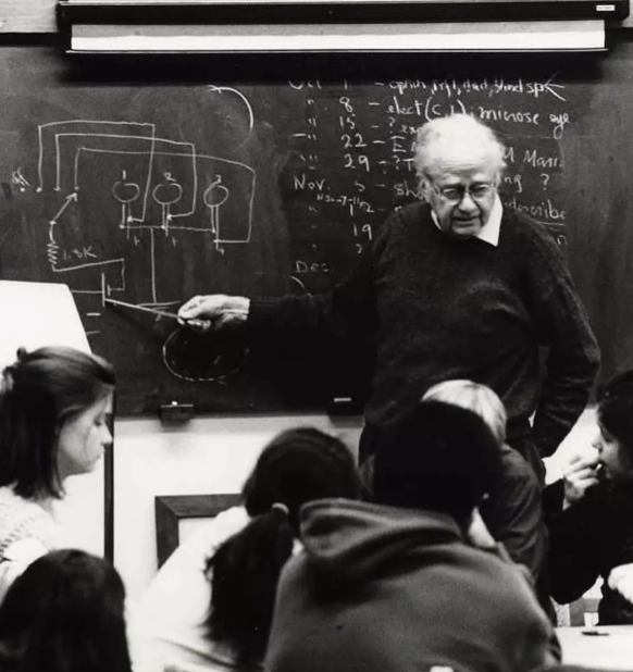
Neurophysiologist. Canadian-born, trained in medicine/research (MD background) and became a leading experimental neuroscientist. Spent most of his career at Harvard Medical School (Department of Neurobiology), working on visual processing in cats and monkeys.

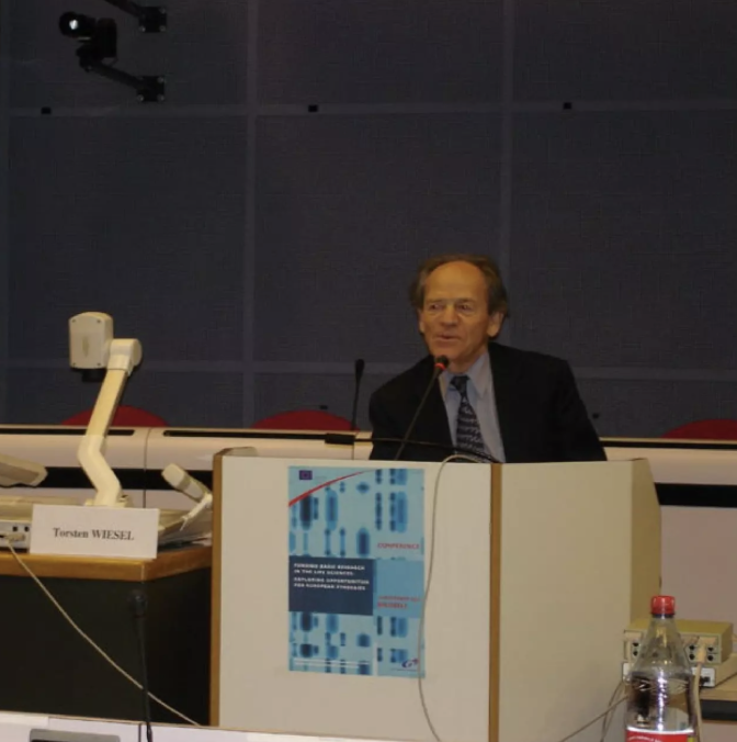
Torsten N. Wiesel (b. 1924):

Neurophysiologist. Swedish-born, medically trained (MD background) and specialized in sensory neurophysiology. Also based at Harvard Medical School during the classic visual cortex work with Hubel.

• Together they ran landmark experiments on the cat’s visual cortex (V1), and they received the 1981 Nobel Prize in Physiology or Medicine (shared) for discoveries about information processing in the visual system

Architecture of visual cortex of the cat

David Hubel

Torsten Wiesel

• Hubel and Wiesel: Cat’s visual cortex
• Recorded from cells in cat V1

Cortex organization

functional architecture of simple cells and complex cells in the early visual cortex

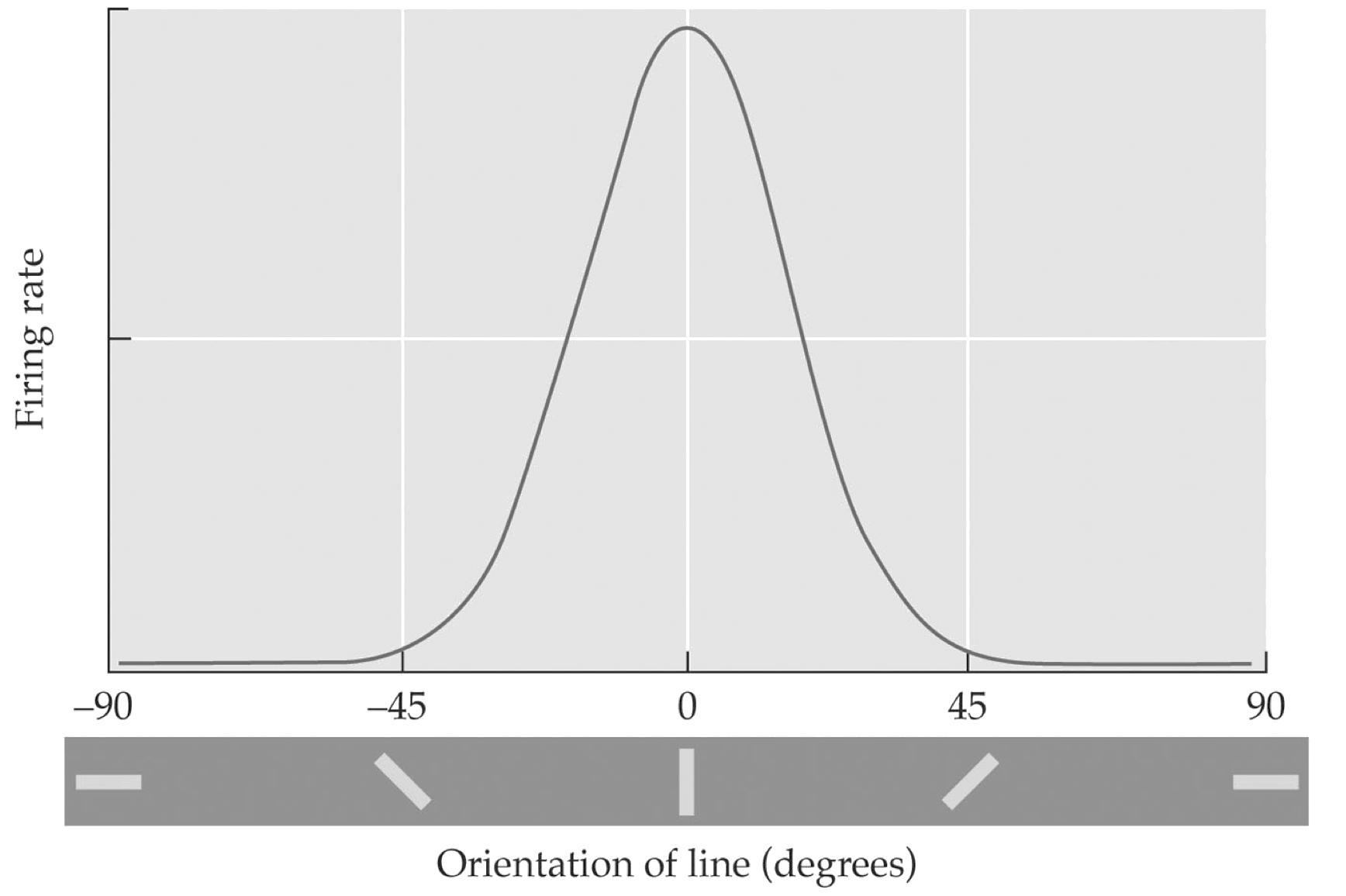
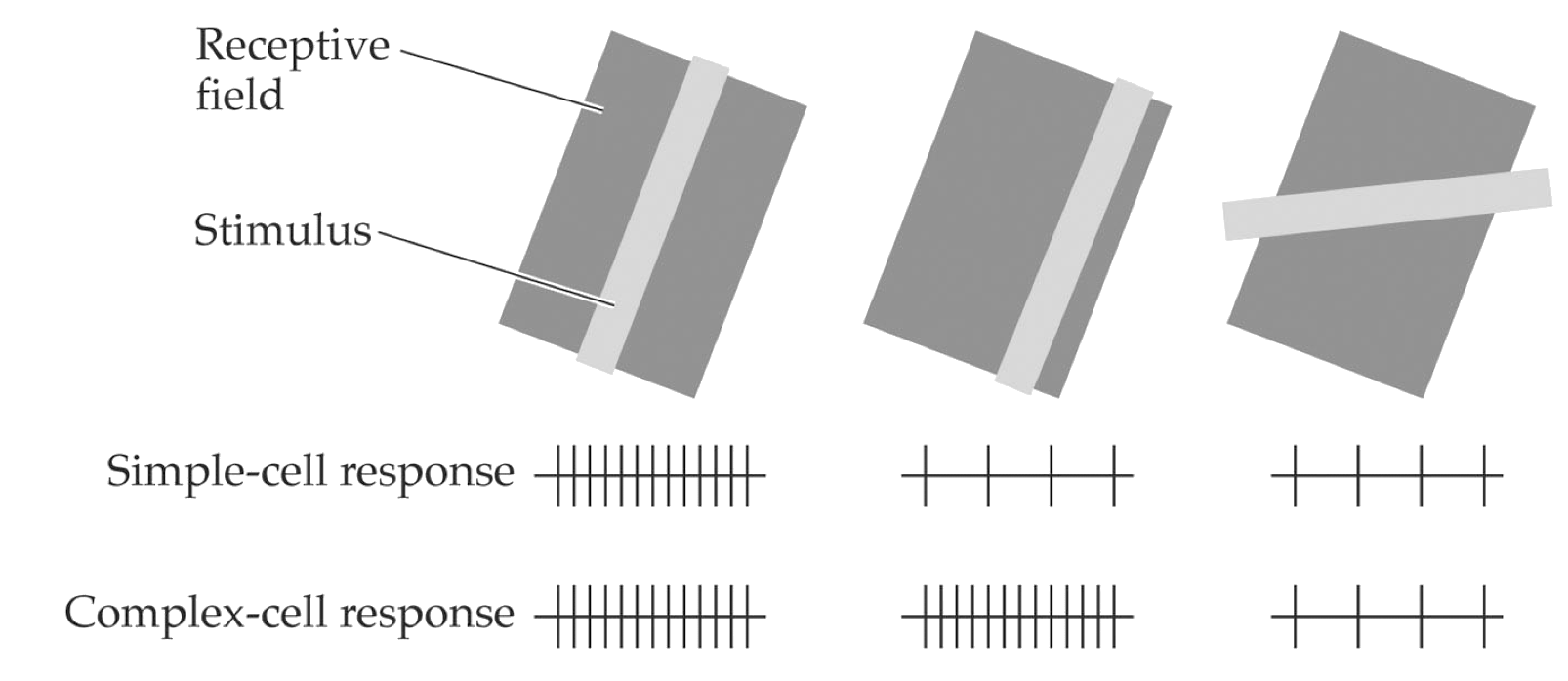
Orientation matters

Orientation Tuning Function of a Cortical Cell

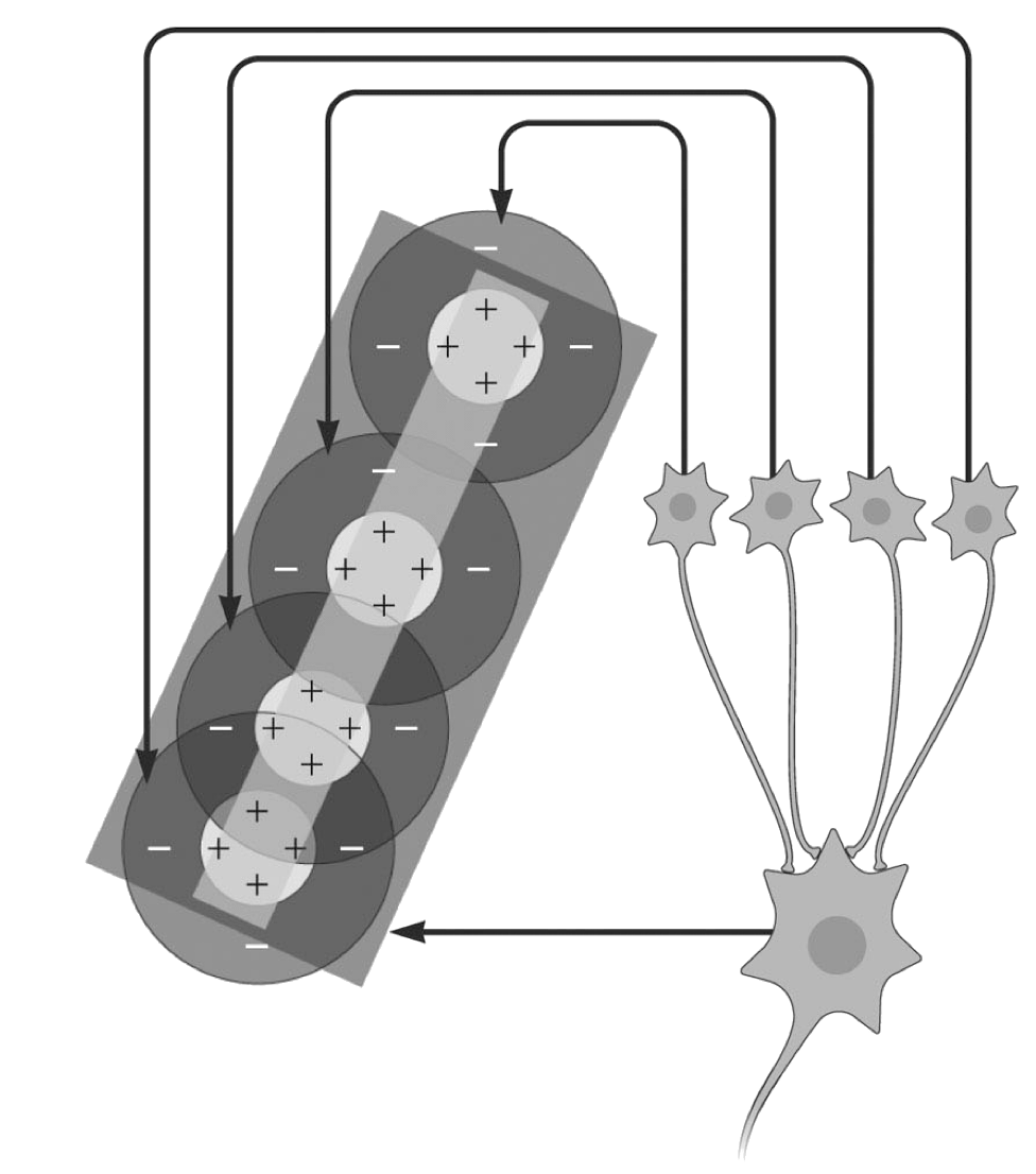
Receptive fields

Receptive Fields in Striate Cortex

• A receptive field is the region of the visual field where a stimulus will change the firing rate of a neuron
• Receptive fields in V1 are small and retinotopic (map the visual field)
• Tend to grow in size with eccentricity, and become more complex through hierarchical pooling of earlier inputs
• V1 neurons respond best to specific local features, especially oriented edges/bars, at a particular location, orientation, spatial frequency, and often motion direction

V1 neurons are the specialized nerve cells in the primary visual cortex (V1) located in the occipital lobe, responsible for the first stage of cortical processing of visual information. They analyze basic features of the visual scene, such as orientation, color, motion, and spatial frequency, providing a detailed map of the visual field.

Receptive fields

Receptive Fields in Striate Cortex

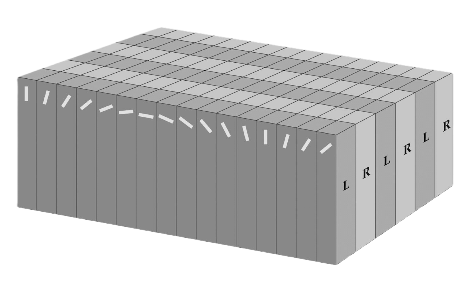
orientation column:

vertical arrangement of neurons – systematic, progressive change in preferred orientation; all orientations were encountered in a distance of about 0.5 mm

hypercolumn:

1-mm block of striate cortex containing:

all the machinery necessary to look after everything the striate cortex is responsible for, in a certain small part of the visual world (Hubel, 1982)

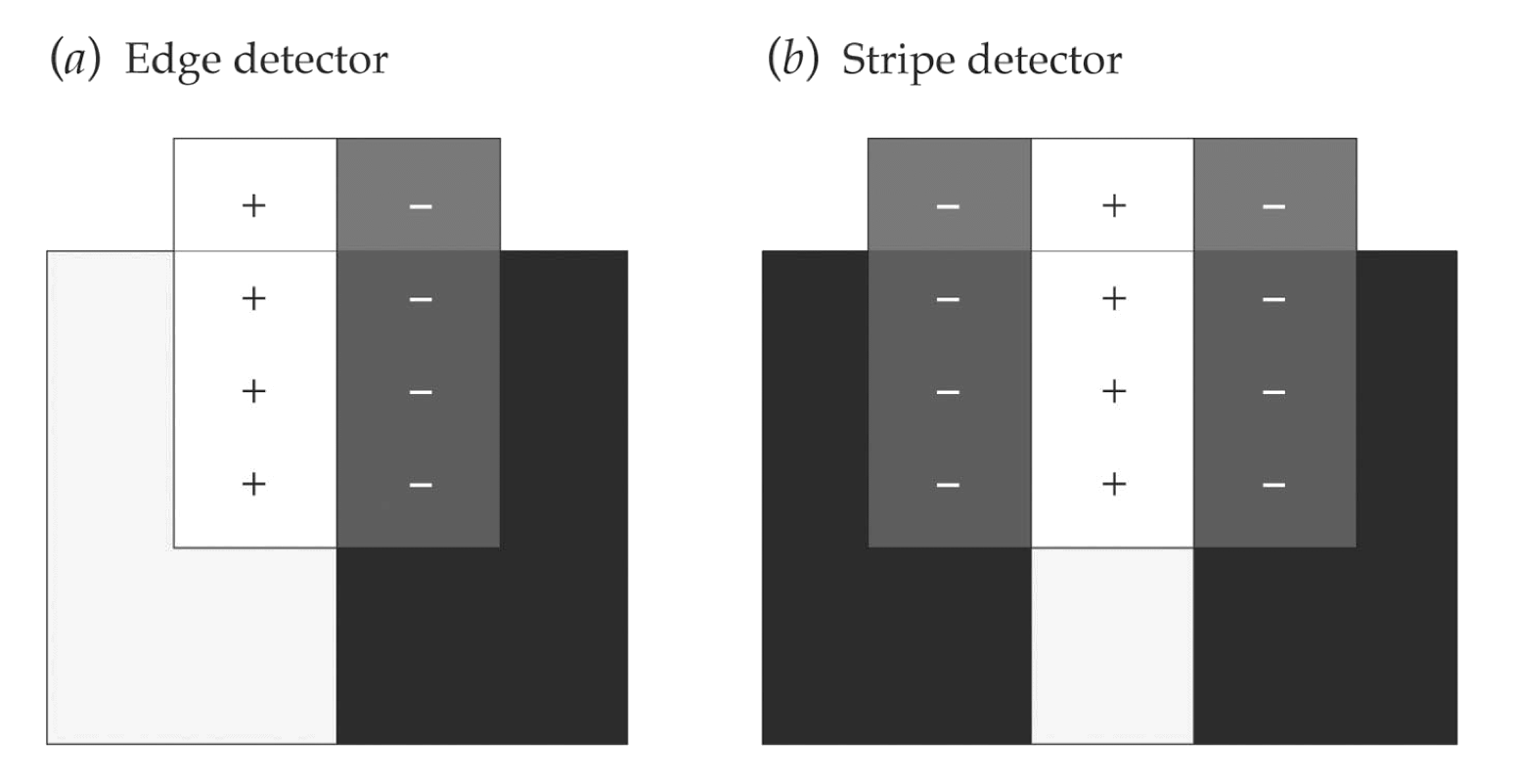
Feature detectors

edge end stripe detectors

Feature detectors

receptive fields vs stimulus

Feature detectors

receptive fields vs stimulus (from Ento Key)

Main findings (V1 / striate cortex)

• Feature-selective receptive fields: many V1 neurons respond best to oriented edges/bars (not spots).
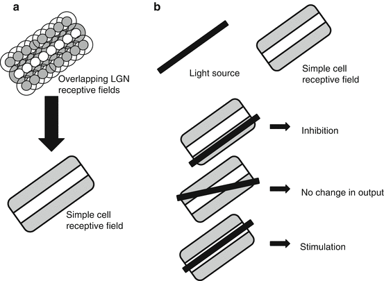
• Cell types:
  • Simple cells: distinct ON/OFF subregions; tuned to position + orientation.
  • Complex cells: orientation-selective but more position-invariant; often direction selective.
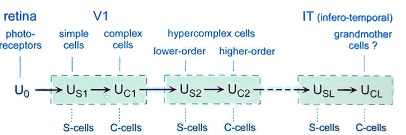
• Hierarchical building blocks: more complex tuning can be explained by pooling simpler inputs (LGN¹ -> simple -> complex).
• Columnar organization: nearby neurons share preferences, forming orientation columns.

Key message: V1 neurons are not “pixel detectors”; they encode local features (orientation, spatial frequency, direction) with increasing invariance from simple -> complex.

1. lateral geniculate nucleus

Cortex organization (maps + columns)

• Retinotopy: V1 contains an orderly map of visual space.
• Ocular dominance: alternating bands biased to left vs right eye input; cells range from monocular to binocular.
• Systematic orientation map: preferred orientation changes smoothly across cortex (later visualized as pinwheel-like patterns).
• Cortex is a structured, modular feature extractor—a blueprint that shaped computational vision and CNN intuition.

Key message: organization is both spatial (retinotopy) and functional (ocular dominance + orientation columns), implying repeated computation across the cortical sheet.

Neocognitron: (Fukushima)

(Fukushima 1980)

Neocognitron: (Fukushima)

• Architecture inspired by the mammalian visual cortex
• A hierarchical, multilayer neural network originally proposed for handwritten character recognition.
• Core promise: recognize learned patterns even when they are partially shifted, rotated, or otherwise distorted.
• Two classical variants are often described:
  • self-organized learning (without a teacher)
  • supervised learning (with a teacher; easier to explain for the core mechanism)

Neocognitron Network Structure

Network Structure

S Layer

S layer

• Feature Detector
• Each cell in the layer detects the presence of a different feature in the layer’s input data
• Adaptable Weights
• Each S-cell is accompanied by a V-cell

s-layer

C Layer

• hiding the exact position of the detected feature
• Improves the network robustness to deformations of the pattern - scaling, shifting of the pattern’s position, or noise

Training

• Weights get initialized with small positive values
• For each training instance, if a cell is the most active in its region and in its plane, then its active weights get reinforced
• Show the same few training instances over and over again
• Math works out so that an S-cell’s weights directly correspond to the feature it is recognizing and activation

Deformation-tolerant recognition

• Unsupervised handwritten character recognition
• The model is designed to output category responses (e.g., “0” vs “1”) even when inputs are not identical to training examples.
• Input - Unlabeled Images
• Output:

Showtime

From https://www.youtube.com/watch?v=oVYCjL54qoY

The “C”

About Images

CS representation of an image

Convolutions

A convolution (denoted by \(*\)) is an operation on two functions \(f\) and \(k\) that produces a third function \((f * k)\).

In machine learning:

• \(f\) is the input
• \(k\) is a kernel
• output is a feature map

A convolutional neural network (CNN) uses convolution in place of general matrix multiplication in at least one layer. (Goodfellow, Bengio, and Courville 2016) It’s main purpose is not dimensionality reduction but feature extraction.

Convolution definition

Definition (continuous and discrete)

Continuous (1D)
\[(f * k)(t) = \int_{-\infty}^{\infty} f(\tau)\,k(t-\tau)\,d\tau\]

Discrete (1D)
\[(f * k)[n] = \sum_{m=-\infty}^{\infty} f[m]\,k[n-m]\]

2D (images)
\[(f * k)[i,j] = \sum_{u}\sum_{v} f[u,v]\,k[i-u,\,j-v]\]

In CNNs, \(f\) is typically a tensor (e.g., height \(\times\) width \(\times\) channels), and \(k\) is learned.

Convolution properties

Commutativity (but…)

Mathematically (under standard conditions):

\[(f * k) = (k * f)\]

But: many deep-learning libraries implement cross-correlation:

\[(f \star k)[n] = \sum_m f[m]\,k[n+m]\]

Cross-correlation differs from convolution by a flip of the kernel index. CNNs still learn filters effectively, but the strict commutativity property doesn’t directly apply to the implemented operator.

Convolution properties

Linearity (superposition)

Convolution is linear in each argument:

• \((a f_1 + b f_2) * k = a(f_1 * k) + b(f_2 * k)\)
  
• \(f * (a k_1 + b k_2) = a(f * k_1) + b(f * k_2)\)

This is one reason convolutions pair naturally with linear algebra operations in neural nets: they preserve additivity and scaling.

Convolution properties

Associativity (stacking filters)

Convolution is associative:

\[ (f * k_1) * k_2 = f * (k_1 * k_2) \]

Interpretation for CNNs:

• If you stack linear convolution layers without nonlinearities, the result is equivalent to a single convolution with an “effective kernel” \(k_{\text{eff}} = k_1 * k_2\).
• In practice, CNNs insert nonlinearities (ReLU, GELU, etc.), so depth adds expressive power beyond a single convolution.

Convolutions properties

Distributive property:

\[ f * (k_1 + k_2) = (f * k_1) + (f * k_2) \]

Identity element: the (Dirac/Kronecker) delta acts like “do nothing”.

• Continuous: \(f * \delta = f\)
  
• Discrete: \(f[n] * \delta[n] = f[n]\) where \(\delta[0]=1\), \(\delta[n\neq 0]=0\)

In CNN terms, an “identity-like” kernel (e.g., a 2D kernel with a 1 in the center and 0 elsewhere) passes features through unchanged.

Convolutions properties

Shift / translation equivariance (key CNN inductive bias)

Let \((T_a f)(t) = f(t-a)\) be a shift operator. Then:

\[ (T_a f) * k = T_a(f * k) \]

So, if the input shifts, the feature map shifts by the same amount: equivariance.

For our CNNs:

• Features (edges, textures) can be detected anywhere using the same kernel.
• Pooling/striding can trade equivariance for approximate invariance (e.g., small translations cause smaller output changes).

Convolutions properties

Differentiation and smoothing

Convolution interacts nicely with derivatives (when everything is well-behaved):

\[ \frac{d}{dt}(f * k) = (f' * k) = (f * k') \]

Classic signal-processing intuition:

• Convolving with a smoothing kernel (e.g., Gaussian) reduces noise.
• Convolving with a derivative-like kernel highlights changes (edges).

CNN filters often learn patterns that resemble smoothing, edge detection, oriented gradients, and more—especially in early layers.

Convolutions properties

Convolution theorem (frequency-domain view)

Let \(\mathcal{F}\) be the Fourier transform. Then:

\[ \mathcal{F}\{f * k\} = \mathcal{F}\{f\}\,\mathcal{F}\{k\} \]

Meaning:

• Convolution in space/time becomes multiplication in frequency.
• \(k\) acts like a frequency response (low-pass, high-pass, band-pass).

Practical CNN angle:

• Some large-kernel convolutions can be computed faster via FFT-based methods, though many modern CNNs rely on highly optimized spatial-domain kernels on GPUs.

Convolutions properties

Separable, dilated, strided, and padded convolutions

Separable kernels: if \(k(x,y)=a(x)b(y)\), then:

\[ f * k = (f * a) * b \]

This can reduce compute (used in depthwise-separable convolutions). (we will see more about this later)

Dilation: increases receptive field without increasing parameters.

Stride: samples the output every \(s\) steps (downsampling).

Padding: controls boundary behavior and output size (“same” vs “valid”).

These variants change how the convolution is applied, but they build on the same core operator.

Convolution properties

Backprop: gradients are (cross-)convolutions too

For a loss \(L\) and output \(y = f * k\), the gradients have convolution structure:

• Gradient w.r.t. input resembles convolution of upstream gradient with a flipped kernel.
• Gradient w.r.t. kernel resembles convolution (or correlation) between the input and upstream gradient.

ok, but what is a convolution?

from https://www.youtube.com/watch?v=KuXjwB4LzSA

Why CNNs are efficient:

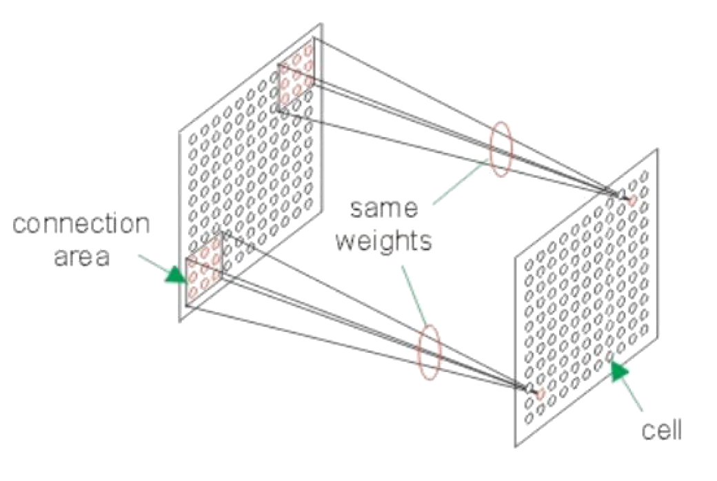
• Parameter sharing: one kernel is reused across positions.
• Local connectivity: kernels are small relative to the input.
• Receptive field growth: stacking layers increases the region of input each output depends on.

Conv 2D

A 2D convolution (Wikimedia)

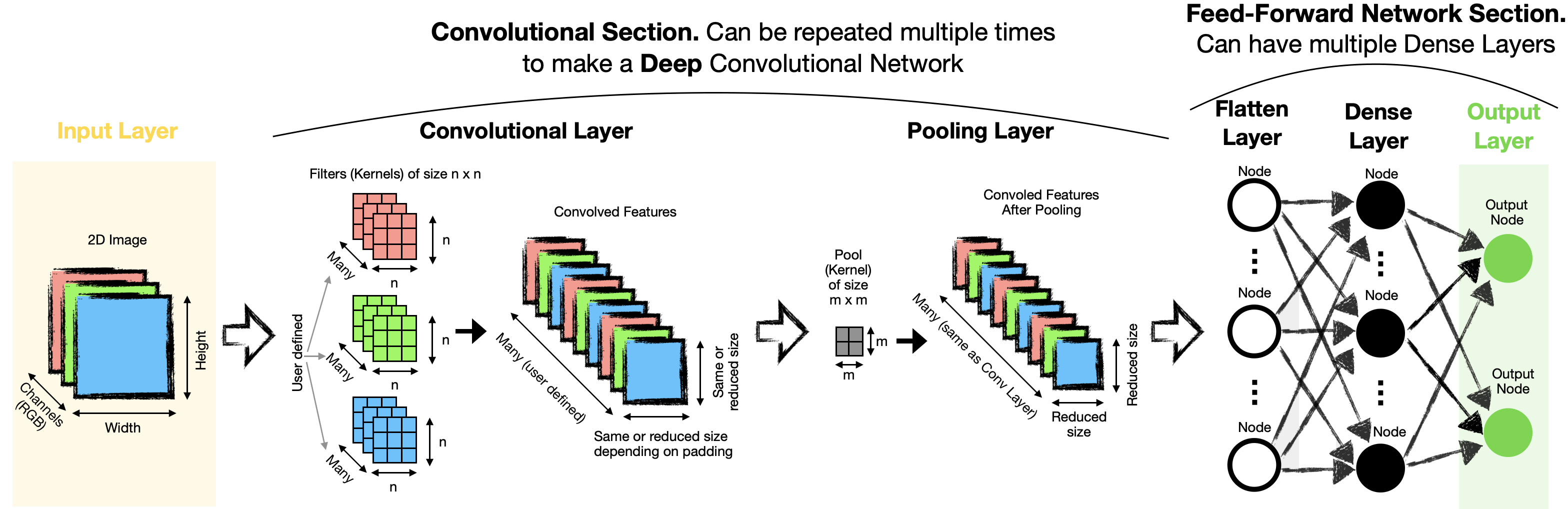
Basic CNN Structure

Three components

• channels
• strides
• padding

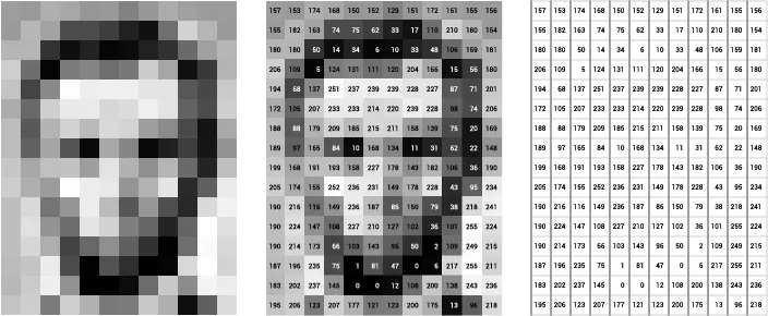
Channels

In color images, pixels intensity are represented a tensori RGB image are formed from the corresponding pixel of the three component

Channels

In color images, pixels intensity are represented a tensori RGB image are formed from the corresponding pixel of the three component

Channels

• A convolution layer applies multiple kernels (filters) to the input.
• Each kernel produces one output channel, also called a feature map.
• The layer’s depth (number of output channels) equals the number of kernels in that layer.
• The full output of the layer is the stack of all feature maps
  
• The shape: (\(H_{out}\), \(W_{out}\), \(K\)) where .
  • (\(H_{out}\)) = the height (number of rows) of each feature map after the convolution
  • (\(W_{out}\)) = the width (number of columns) of each feature map after the convolution
  • (\(K\)) = the number of feature maps, i.e., the number of kernels/filters in the layer So you can think of it as (K) separate 2D images, each of size (H\(_{out} \times W_{out}\)), stacked along the “channel” dimension.

Example: if a layer outputs (\(H_{out}\)=32), (\(W_{out}\)=32), and you use (\(K=64\)) filters, the output shape is (32, 32, 64): 64 feature maps, each 32×32.

Strides

• Stride = step size of the kernel as it slides across the input.
• If S = 1, the kernel moves 1 cell/pixel at a time -> dense output (more positions).
• If S = 2, it moves 2 cells/pixels at a time -> smaller output (downsampling).
• Bigger stride -> fewer kernel positions -> smaller \(H_{out}\), \(W_{out}\) and less computation.

Intuition: stride controls how many places you evaluate the filter. Larger stride skips positions and reduces spatial resolution.

Padding

• Padding = adding extra border cells (usually zeros) around the input before applying the kernel.
• Main purpose: control output size and preserve information at the edges of the image.
• With \(P=0\) (“valid” conv): output shrinks because the kernel can’t go outside the input.
• With \(P>0\) (often “same” conv when combined with \(S=1\)): output can keep similar spatial size, and border pixels influence more outputs.

Padding lets filters “see” the border properly and prevents rapid shrinking of \(H_{out}, W_{out}\) across layers.

Convolution output size (1D)

\[ \text{Output size} \;=\; \left\lfloor \frac{\text{Input size} + 2P - K}{S} \right\rfloor + 1 \]

• Input size: number of positions in the input (e.g., width in 1D, or width/height in 2D).
• \(P\) (padding): adds \(P\) cells on each side, so total added is \(2P\).
• \(K\) (kernel size): the kernel must “fit” inside the padded input, so we subtract \(K\).
• \(S\) (stride): step size of the kernel; dividing by \(S\) counts how many valid steps fit.
• \(\lfloor \cdot \rfloor\) (floor): if it doesn’t divide evenly, we keep only the complete steps.
• \(+1\): counts the first kernel position (at the start).

For 2D, apply the same formula separately to height and width: \(H_{out}=\left\lfloor\frac{H+2P-K}{S}\right\rfloor+1\), \(W_{out}=\left\lfloor\frac{W+2P-K}{S}\right\rfloor+1\).

Convolution output size (2D)

It applies to 2D per dimension.

For an input of size \(H \times W\) (height × width), kernel \(K_h \times K_w\), padding \(P_h, P_w\), stride \(S_h, S_w\):

\[ H_{\text{out}}=\left\lfloor \frac{H+2P_h-K_h}{S_h}\right\rfloor + 1 \qquad W_{\text{out}}=\left\lfloor \frac{W+2P_w-K_w}{S_w}\right\rfloor + 1 \]

If you use the common symmetric case (\(K_h=K_w=K\), \(P_h=P_w=P\), \(S_h=S_w=S\)), it’s the same formula applied to both \(H\) and \(W\)

Better and image

Input Size

Padding

Kernel Size

Stride

Input (7, 7)

After-padding (7, 7)

🖱️ Hover over the matrices to change kernel position.

Output (3, 3)

 

Between the “C” and the “NN”

Pooling layers (Max/Average Pooling)

• Replaces each local window (e.g., \(2\times2\)) with one value
  • Max pooling: keeps the largest value
    
  • Average pooling: takes the mean
• They reduce spatial size (\(H, W\)):
  • less computation
  • less overfitting
  • robustness to small shifts.
• Pooling typically reduces \(H\) and \(W\), but keeps the number of channels \(K\) the same.
• Example: with a \(2\times2\) window and stride \(2\), an input \((32,32,K)\) becomes \((16,16,K)\).

Pooling is like “summarizing” nearby activations. It increases translation tolerance, but too much pooling can discard detail.

Pooling layer

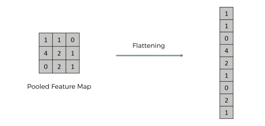
Flatten layer

• Converts a multi-dimensional tensor into a 1D vector (per example), without changing the values.
• Typical use: between convolution/pooling blocks and a fully connected (dense) layer.
• Example shape change:
  • Input: \((H, W, K) = (8, 8, 32)\)
  • Output: \((8 \cdot 8 \cdot 32) = (2048)\)
• Flatten has no learnable parameters — it’s just a reshape.

Flatten doesn’t “extract features”; it reorganizes them so dense layers can operate on a single vector.

Flatten layer

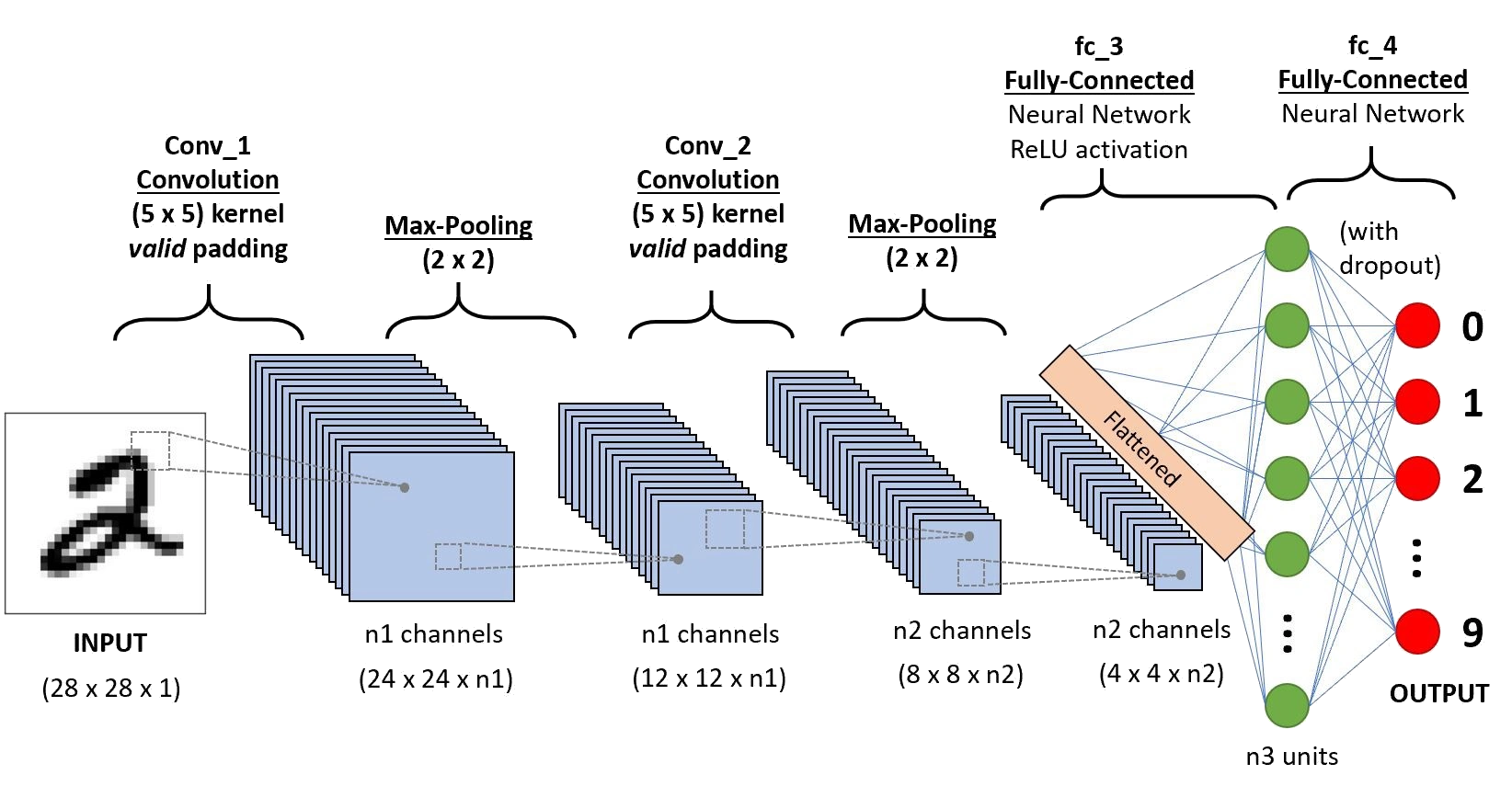
All together

“The” CNNs

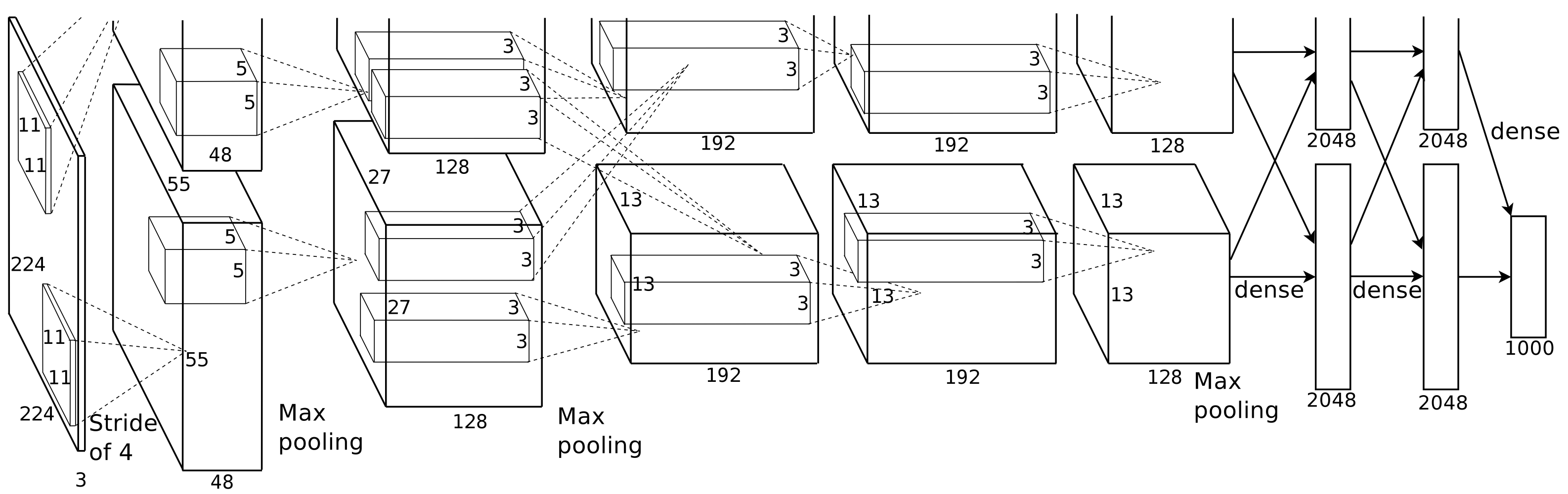
AlexNet (ImageNet Contest 2012)

• Winner of ImageNet Large Scale Visual Recognition Challenge (ILSVRC) 2012
• ImageNet:
  • 15+ million labeled high-resolution images
  • 22000 categories ILVRC subset:
  • 1000 images per category
  • 1000 categories
  • 1.2 million training images | 50000 validation images | 150000 testing images

AlexNet Task

An illustration of the architecture of our CNN explicitly showing the delineation of responsibilities between the two GPUs. One GPU runs the layer-parts at the top of the figure while the other runs the layer-parts at the bottom. The GPUs communicate only at certain layers The network’s input is 150,528-dimensional, and the number of neurons in the network’s remaining layers is given by 253,440–186,624–64,896–64,896–43,264–4096–4096–1000.

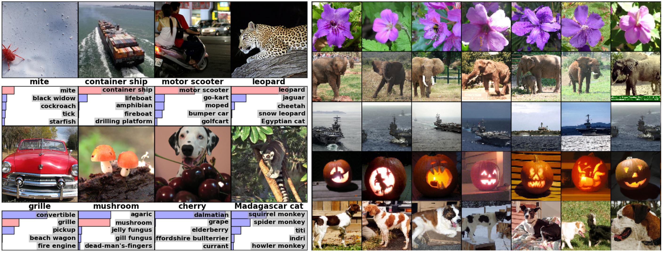
AlexNet Task

(Left) Eight ILSVRC-2010 test images and the five labels considered most probable by our model. The correct label is written under each image, and the probability assigned to the correct label is also shown with a red bar (if it happens to be in the top 5). (Right) Five ILSVRC-2010 test images in the first column The remaining columns show the six training images that produce feature vectors in the last hidden layer with the smallest Euclidean distance from the feature vector for the test image.

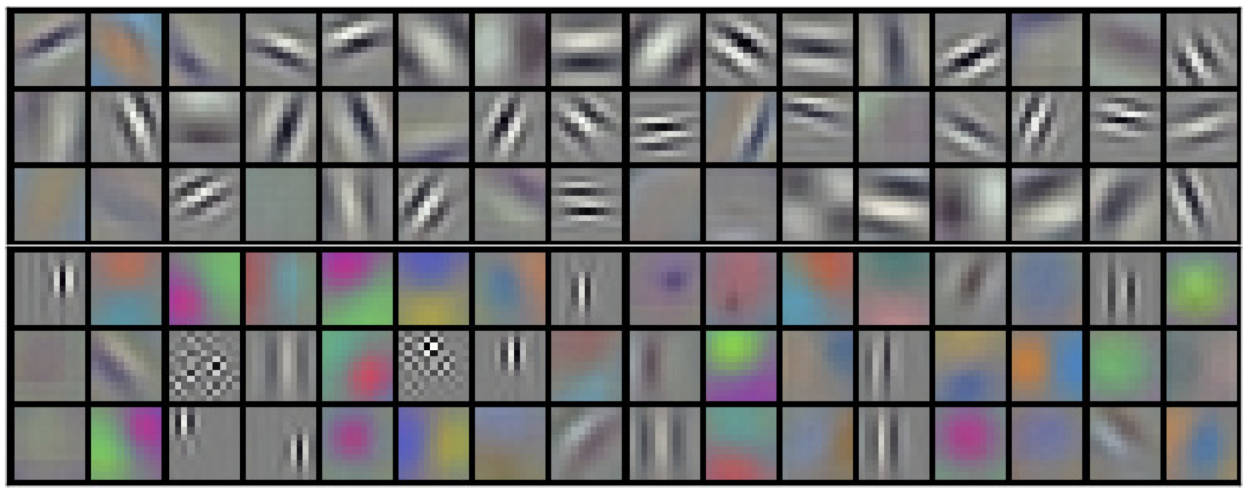
AlexNet kernels

96 convolutional kernels of size 11×11×3 learned by the first convolutional layer on the 224×224×3 input images. The top 48 kernels were learned on GPU 1 while the bottom 48 kernels were learned on GPU 2

Local Response Normalization LRN

AlexNet introduced LRN to mimic a form of lateral inhibition (biological inspiration). The idea is to encourage competition between neighboring feature maps at the same spatial location.:

• If several channels respond strongly at the same pixel, they suppress each other.
• This makes the most strongly activated feature maps stand out.

Motivation in 2012 context:

• ReLU activations can produce large responses.
• LRN provided extra regularization/stabilization when training deep CNNs on ImageNet.

Local Response Normalization (LRN)

AlexNet used a LRN technique.

Given an activation \(a_{x,y}^i\) at position \((x,y)\) in channel \(i\), LRN outputs:

\[ \underbrace{b_{x,y}^i}_{\text{normalized response}} = \underbrace{a_{x,y}^i}_{\text{activation (after ReLU)}} / \left( \underbrace{k}_{\text{bias}} + \underbrace{\alpha}_{\text{scaling}} \sum_{j\in\mathcal{N}(i)} (\underbrace{a_{x,y}^j}_{\text{neighboring channels}})^2 \right)^{\beta} \]

• \(N\): number of channels (feature maps)\(\mathcal{N}(i)=\{j:\;|j-i|\le n/2\}\cap[0,N-1]\)
• \(n\): size of the local neighborhood across channels
• Typical AlexNet hyperparams: \(k=2\), \(n=5\), \(\alpha=10^{-4}\), \(\beta=0.75\)

Effect in AlexNet

LRN is applied after ReLU in AlexNet (in the early conv layers).

Observed effect:

• Small but measurable improvement in ImageNet accuracy.
• Encourages sparser / more selective channel responses.

Trade-offs:

• Adds computation and extra hyperparameters.
• Later architectures (VGG/ResNet) largely dropped LRN in favor of better regularization and normalization (e.g., BatchNorm).

CNN explainer

See it at:

• https://www.youtube.com/watch?v=HnWIHWFbuUQ
• https://poloclub.github.io/cnn-explainer

from (POLO Club 2019; Wang et al. 2021)

Applications, general overview

In the domain of Bioinformatics

• Biomedical imaging (cells, tissues, organs)
• High-content screening and microscopy phenotyping
• Computational pathology whole slide image (WSI)
• CNNs 1D convolutions on sequences (Alipanahi et al. 2015; Zhou and Troyanskaya 2015)
• CNNs 1D convolutions on biomedical signals (ECG,EEG) (Alipanahi et al. 2015; Zhou and Troyanskaya 2015)

Biomedical imaging

Modality	Typical data	Key quirks	Common CNN strategy
Histopathology (WSI)	Gigapixel slides	stain variation, tiling, weak labels	MIL / tile CNN + aggregation
Microscopy	cells/tissues	illumination, blur, small objects	U-Net/Mask R-CNN, augmentations
Radiology (CT/MRI/X-ray)	2D/3D volumes	anisotropy, 3D context	2.5D/3D CNNs, careful splits
Physiological signals (ECG/EEG/EMG)	1D time series (multi-lead / multi-channel), sometimes transformed to time–frequency	nonstationarity, noise/artifacts (motion, baseline wander), variable length, subject/device variability, label ambiguity (event timing)	1D CNN / TCN on raw or filtered signals; windowing + stride; multi-channel convolutions; often add spectrograms (STFT/wavelets) -> 2D CNN; patient-wise splits, augmentation (jitter, scaling, time-warp), class-imbalance handling

Leakage risk differs: in WSI, multiple tiles from one slide; in radiology, multiple slices per patient.

Classification tasks in biomed (examples)

• Disease detection / grading (e.g., skin lesions, diabetic retinopathy, cancer subtyping)
• Cell phenotype classification (immune cell states, mitosis detection)
• Subcellular localization (protein patterns)
• Parasite/organism identification in microscopy
• Drug response phenotyping in screening plates

Classification: patch/tiling vs whole-image

• Whole image works for modest-sized images (microscopy tiles, X-rays)
• Whole-slide images (WSI) require tiling
  • Extract patches at one or more magnifications
  • Run CNN per tile
  • Aggregate to slide/patient prediction (max/mean/attention/MIL)

Semantic vs instance segmentation

• Semantic segmentation: each pixel gets a class (cell vs background)
• Instance segmentation: separate objects (each cell/nucleus gets its own ID)
  • Mask R-CNN-style approach (He et al. 2017)
  • or post-processing on semantic maps (watershed, connected components)

Weak supervision for WSI (common)

• Labels often at slide level, not pixel/region level
• Strategy:
  • train tile encoder \(f_\theta(x_i)\rightarrow z_i\)
  • aggregate to slide score \(\hat{y}=g(\{z_i\})\)
• Practical aggregation choices:
  • top-\(k\) pooling, attention pooling, mean pooling
• Case study later: weakly supervised WSI pathology (Campanella et al. 2019)

Hematoxylin & Eosin (H&E) staining

• H&E most common routine stain in histology.
• It combines two dyes:
  • Hematoxylin (with a mordant) stains basophilic structures -> mainly cell nuclei (blue/purple)
  • Eosin stains eosinophilic structures -> mainly cytoplasm and extracellular proteins (pink)
• Viewing tissue structure under a light microscope shows strong contrast between nuclei vs cytoplasm/ECM so tissue architecture is easy to interpret.

A mordant is a chemical “fixer” that binds a dye to tissue and makes the staining stronger and more stable.

• In H&E, hematoxylin by itself doesn’t bind strongly to nuclei. It’s typically used with a metal mordant (commonly aluminum or iron salts).
• The mordant forms a dye–metal complex (often called a lake) that has high affinity for basophilic/negatively charged structures like DNA/RNA in nuclei.
• Result: sharper, more permanent nuclear staining (blue/purple), improving contrast against eosin-stained cytoplasm/ECM (pink).

Histopathology specifics: stain & color

• Hematoxylin and eosin (H&E) staining accounts for over 80% of slides stained worldwide
• Stain variability (H&E) causes domain shift
• Common fixes:
  • color augmentation
  • stain normalization methods
  • multi-site training + validation
• Avoid “too-clean” preprocessing that removes diagnostic cues

Histopathology specifics: stain & color inference

Histochemical staining of H&E is digitally transformed using a deep neural network into the special stains: (i) generation of JMS (purple arrow); (ii) generation of MT (Masson’s Trichrome, red arrow); (iii) generation of PAS (Periodic acid–Schiff, blue arrow).

from (Haan et al. 2021)

They start with a standard H&E slide (the routine stain). - A deep neural network takes the digital image of that H&E slide and computationally converts it into images that look like (and aim to mimic the information of) other special stains—without physically re-staining the tissue. - The network generates three “virtual stains”: 1. JMS (often written JMS/Jones stain) — commonly used to highlight basement membranes (e.g., in kidney pathology). (purple arrow points to this output) 2. MT = Masson’s Trichrome — highlights collagen/fibrosis (connective tissue) versus muscle/cytoplasm. (red arrow) 3. PAS = Periodic acid–Schiff — highlights carbohydrates/glycoproteins, e.g., mucins and basement membranes. (blue arrow)

U-Net for biomedical segmentation

U-Net: Convolutional Networks for Biomedical Image Segmentation

• Dense, pixelwise prediction with precise localization from limited labeled data (Ronneberger, Fischer, and Brox 2015a, 2015b).
• Key idea: encoder–decoder with skip connections that transfer high-resolution features directly to matching decoder stages.
• Practical focus:
  • strong data augmentation (esp. elastic deformations),
  • careful handling of borders and class imbalance,
  • fast inference on full images via tiling/overlap.

Architecture (the “U”)

• Contracting path: repeated \(3\times 3\) conv + nonlinearity, then downsampling (context aggregation).
• Expanding path: upsampling + conv (localization refinement).
• Skip connections concatenate encoder features into the decoder at the same spatial scale.

Skip connections as multiscale feature fusion

Let the encoder feature map at level \(\ell\) be \(E_\ell \in \mathbb{R}^{H_\ell \times W_\ell \times C_\ell}\) and the decoder feature map before fusion be \(D_\ell \in \mathbb{R}^{H_\ell \times W_\ell \times C'_\ell}\).

• Upsample decoder features: \(\tilde{D}_\ell = \mathrm{Up}(D_{\ell+1})\)
• Fuse via channel-wise concatenation: \[ F_\ell = \mathrm{Concat}\big(E_\ell,\ \tilde{D}_\ell\big) \]
• Then refine: \[ D_\ell = g_\ell(F_\ell) \] where \(g_\ell(\cdot)\) denotes the conv block at level \(\ell\).

Concatenation preserves fine spatial cues in \(E_\ell\) while \(\tilde{D}_\ell\) carries semantic context from deeper layers, improving boundary localization (Ronneberger, Fischer, and Brox 2015a).

Pixelwise prediction + weighted loss for borders

For each pixel \(x\) and class \(k\), logits \(a_k(x)\) produce softmax probabilities: \[ p_k(x) = \frac{\exp(a_k(x))}{\sum_{k'=1}^{K}\exp(a_{k'}(x))} \]

U-Net uses a weighted pixelwise cross-entropy to emphasize difficult regions (notably touching objects / borders): \[ \mathcal{L} = -\sum_{x\in\Omega} w(x)\,\log\big(p_{y(x)}(x)\big) \] where \(y(x)\) is the ground-truth class at pixel \(x\), and \(w(x)\) is a precomputed weight map that upweights separation boundaries (Ronneberger, Fischer, and Brox 2015a, 2015b).

U-Net Training & inference details

• Data augmentation: heavy geometric + photometric augmentation; elastic deformations are highlighted as especially effective for biomedical imagery (Ronneberger, Fischer, and Brox 2015a).
• Valid vs. same padding: original U-Net uses valid convolutions, shrinking spatial size; output is produced for the central region of a larger input patch.
• Inference on large images: tile the image, predict per tile, and blend overlaps to reduce boundary artifacts.
• Strong benchmark performance on ISBI-style biomedical tasks and robust results with few training images (Ronneberger, Fischer, and Brox 2015a).

Pitfalls and others

Main pitfalls (the stuff that breaks papers)

• Data leakage
  • tiles from same WSI across train/test
  • slices from same patient across splits
• Batch/site effects
  • scanner differences, staining labs, acquisition protocols
• Annotation noise
  • weak labels, inter-rater variability, ambiguous boundaries
• Hidden stratification
  • model “works” overall but fails on rare clinically important subtypes

Questions

References

Alipanahi, Babak, Andrew Delong, Matthew T. Weirauch, and Brendan J. Frey. 2015. “Predicting the Sequence Specificities of DNA- and RNA-Binding Proteins by Deep Learning.” Nature Biotechnology 33 (8): 831–38. https://doi.org/10.1038/nbt.3300.

Campanella, Gabriele, Michael G. Hanna, Lucian Geneslaw, Adrian Miraflor, Victor Werneck Krauss Silva, Klaus J. Busam, Edi Brogi, Victor E. Reuter, David S. Klimstra, and Thomas J. Fuchs. 2019. “Clinical-Grade Computational Pathology Using Weakly Supervised Deep Learning on Whole Slide Images.” Nature Medicine 25: 1301–9. https://doi.org/10.1038/s41591-019-0508-1.

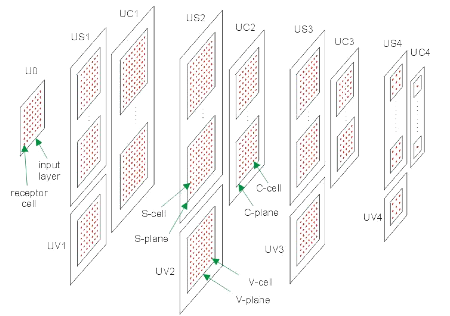
Fukushima, Kunihiko. 1980. “Neocognitron: A Self-Organizing Neural Network Model for a Mechanism of Pattern Recognition Unaffected by Shift in Position.” Biological Cybernetics 36 (4): 193–202. https://doi.org/10.1007/BF00344251.

Goodfellow, Ian, Yoshua Bengio, and Aaron Courville. 2016. Deep Learning. MIT Press.

Haan, Koen de, Yair Zhang, Joseph E. Zuckerman, Tianyu Liu, Ashley E. Sisk, MFP Diaz, Kun Y. Jen, et al. 2021. “Deep Learning-Based Transformation of h&e Stained Tissues into Special Stains.” Nature Communications 12 (1): 4884. https://doi.org/10.1038/s41467-021-25221-2.

He, Kaiming, Georgia Gkioxari, Piotr Dollár, and Ross Girshick. 2017. “Mask r-CNN.” In Proceedings of the IEEE International Conference on Computer Vision (ICCV), 2961–69. https://doi.org/10.1109/ICCV.2017.322.

He, Kaiming, Xiangyu Zhang, Shaoqing Ren, and Jian Sun. 2016. “Deep Residual Learning for Image Recognition.” In Proceedings of the IEEE Conference on Computer Vision and Pattern Recognition (CVPR), 770–78. https://doi.org/10.1109/CVPR.2016.90.

Ioffe, Sergey, and Christian Szegedy. 2015. “Batch Normalization: Accelerating Deep Network Training by Reducing Internal Covariate Shift.” In Proceedings of the 32nd International Conference on Machine Learning (ICML), 37:448–56. Proceedings of Machine Learning Research. PMLR. http://proceedings.mlr.press/v37/ioffe15.html.

Krizhevsky, Alex, Ilya Sutskever, and Geoffrey E. Hinton. 2012. “ImageNet Classification with Deep Convolutional Neural Networks.” In Advances in Neural Information Processing Systems. Vol. 25. https://papers.nips.cc/paper/2012/hash/c399862d3b9d6b76c8436e924a68c45b-Abstract.html.

LeCun, Yann, Bernhard Boser, John S. Denker, Donnie Henderson, Richard E. Howard, Wayne Hubbard, and Lawrence D. Jackel. 1989. “Backpropagation Applied to Handwritten Zip Code Recognition.” Neural Computation 1 (4): 541–51. https://doi.org/10.1162/neco.1989.1.4.541.

LeCun, Yann, Léon Bottou, Yoshua Bengio, and Patrick Haffner. 1998. “Gradient-Based Learning Applied to Document Recognition.” In Proceedings of the IEEE, 86:2278–2324. 11. IEEE. https://doi.org/10.1109/5.726791.

POLO Club. 2019. “CNN Explainer.” https://poloclub.github.io/cnn-explainer/.

Ronneberger, Olaf, Philipp Fischer, and Thomas Brox. 2015a. “U-Net: Convolutional Networks for Biomedical Image Segmentation.” https://arxiv.org/abs/1505.04597.

———. 2015b. “U-Net: Convolutional Networks for Biomedical Image Segmentation.” In Medical Image Computing and Computer-Assisted Intervention – MICCAI 2015, edited by Nassir Navab, Joachim Hornegger, William M. Wells, and Alejandro F. Frangi, 9351:234–41. Lecture Notes in Computer Science. Springer, Cham. https://doi.org/10.1007/978-3-319-24574-4_28.

Simonyan, Karen, and Andrew Zisserman. 2015. “Very Deep Convolutional Networks for Large-Scale Image Recognition.” In International Conference on Learning Representations (ICLR). https://arxiv.org/abs/1409.1556.

Wang, Zijie J., Robert Turko, Omar Shaikh, Haekyu Park, Nilaksh Das, Fred Hohman, Minsuk Kahng, and Duen Horng Polo Chau. 2021. “CNN Explainer: Learning Convolutional Neural Networks with Interactive Visualization.” IEEE Transactions on Visualization and Computer Graphics 27 (2): 1396–406. https://doi.org/10.1109/tvcg.2020.3030418.

Zhou, Jian, and Olga G. Troyanskaya. 2015. “Predicting Effects of Noncoding Variants with Deep Learning–Based Sequence Model.” Nature Methods 12 (10): 931–34. https://doi.org/10.1038/nmeth.3547.

Extra slides !!

• Slides extra which are always nice to have