Sequence analysis

Motivation

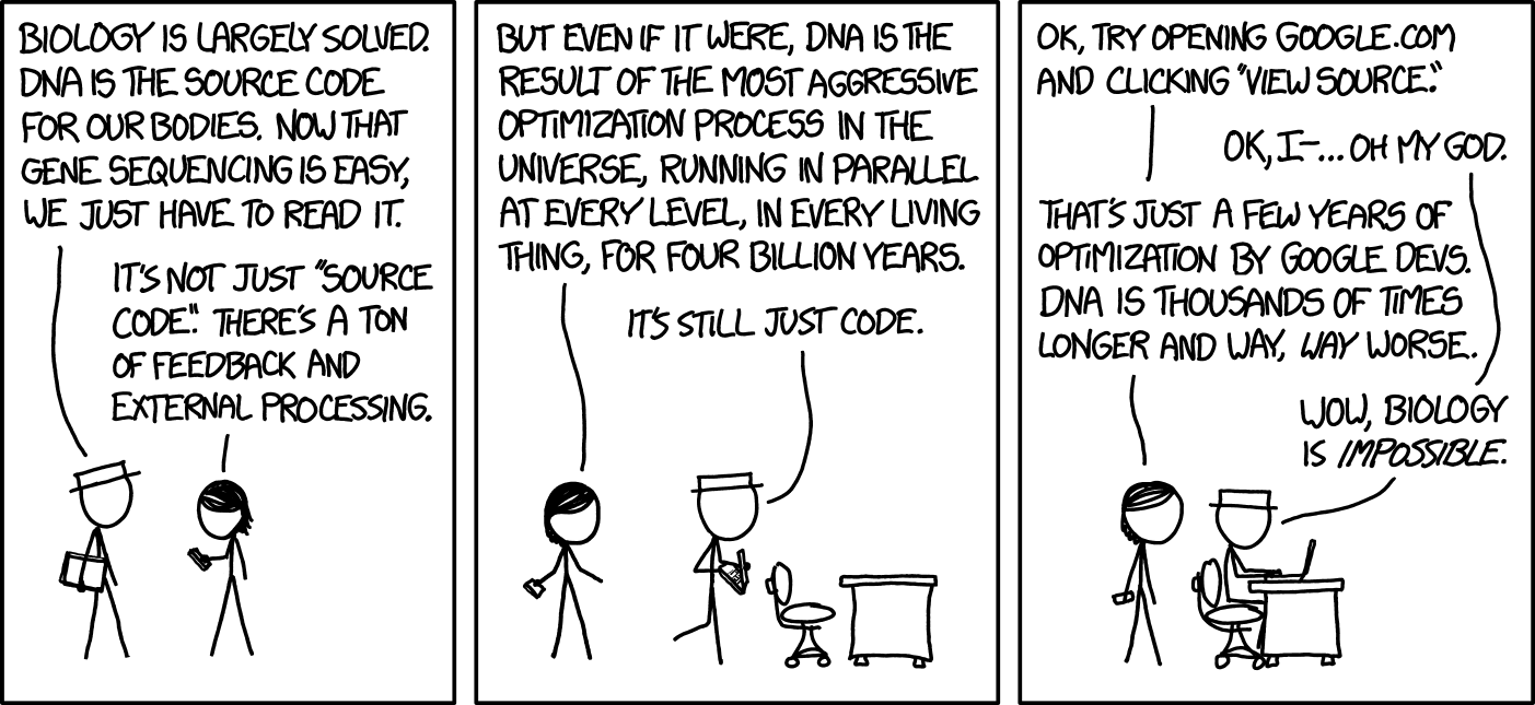
Cartoon: 'Biology is largely solved. DNA is the source code for our bodies.' — 'Try opening google.com and clicking view source… oh my god.' — 'Biology is impossible.'

xkcd 1605 “DNA” — Randall Munroe, xkcd.com/1605, CC BY-NC 2.5.

Motivation

Prediction of biological and structural properties from sequences is a key goal in computational biology.

Recognise transmembrane proteins from sequence alone (about 25% of all proteins).
Classify proteins into classes of similar function from sequence similarity.
These proteins mediate communication and transport between cells, and are central to recent pharmaceutical developments.

Sequence Analysis

Per-Sequence Analysis

Limited information.
Analyzed solely from sequence information (residues).
Characteristics of residues
- Physical, chemical: hydrophobicity (amino acids)
- Statistical: GC islands (DNA); codon usage

Between Sequences

More informative.
Mainly based on homology.
Common ancestry and sequence similarity.
Homology indicates common ancestry. Shared function requires additional evidence.
The base of homology recognition is the similarity concept between two sequences.
Genes come in families -> multiple sequence analysis.

Profiles

Amino acid Features

Size.
Flexibility in the backbone.
Charge.
…

Argos

Argos (1987). A sensitive Procedure to Compare Amino acid Sequences. J. Mol. 193:385-396

Hydrophobicity.
Turn Preference.
Residue Bulk or Shape.
Refractivity Index.
Antiparallel strand preference.

Most computed in a sliding window approach.

Sequence profiles

Features on individual amino acids play some role in protein early secondary structure formation

Glutamate is frequently found in alpha helices
Valine has a preference for beta strands.
Proline is strongly avoided in helices

Sequence profiles

Hydrophobicity scales

Hydrophobicity

Physico-chemical property

Kyte-Doolittle

Widely applied scale for delineating hydrophobic character of a protein. with values above 0 are hydrophobic in character.

Hopp-Woods

Designed for predicting potentially antigenic regions.
Values greater than 0 are hydrophilic and thus likely to be exposed on the surface of a folded protein.

Both are computed on a sliding window, like the Argos profiles above.

Hydrophobicity: the two scales side by side

	Kyte-Doolittle	Hopp-Woods
Alanine	1.8	-0.5
Arginine	-4.5	3.0
Asparagine	-3.5	0.2
Aspartic acid	-3.5	3.0
Cysteine	2.5	-1.0
Glutamine	-3.5	0.2
Glutamic acid	-3.5	3.0
Glycine	-0.4	0.0
Histidine	-3.2	-0.5
Isoleucine	4.5	-1.8

	Kyte-Doolittle	Hopp-Woods
Leucine	3.8	-1.8
Lysine	-3.9	3.0
Methionine	1.9	-1.3
Phenylalanine	2.8	-2.5
Proline	-1.6	0.0
Serine	-0.8	0.3
Threonine	-0.7	-0.4
Tryptophan	-0.9	-3.4
Tyrosine	-1.3	-2.3
Valine	4.2	-1.5

Values from Black, S.D. and Mould, D.R. (1991) Anal. Biochem. 193, 72–82. Sign conventions differ: Kyte-Doolittle > 0 marks hydrophobic residues; Hopp-Woods > 0 marks hydrophilic, exposed ones.

Hydrophobicity Profiles

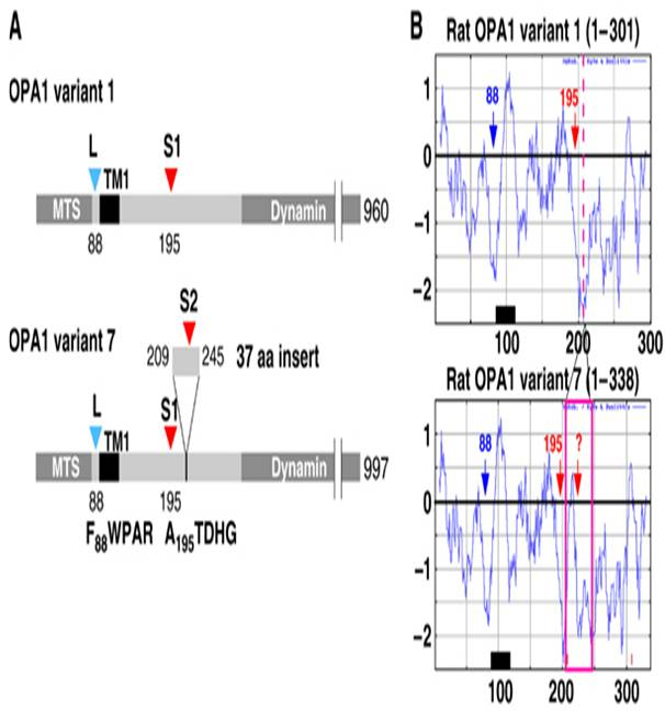
Rat OPA1 windowed hydropathy: TM1 (≈residue 100) is the only clear hydrophobic peak; variant 7 adds a 37-aa hydrophilic insert.

Pairwise alignment

Evolution suggests

All gene sequences may have derived from common ancestral sequences.
Trace the evolutionary history of mutations will help us to understand functionality and structure

Comparing two sequences

Which is this mutation path, using:
- Insertions.
- Deletions.
- Mutations.
… to turn a sequence into another?

Distance between sequences.

Why is it useful?

May provide information whether sequence contains protein-coding gene.
Similarity on sequence may hint first clues on the type of protein the gene codes.
Protein Structure Prediction.
Compare DNA information between organisms -> Phylogenetic tree.

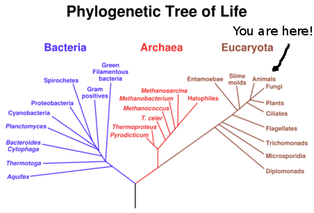
Phylogenetic Tree of Life

Phylogenetic Tree of Life, with a 'You are here!' tag on the Eucaryota branch

Based on 16S rRNA genetic sequences. Woese C, Fox G (1977).”Phylogenetic structure of the prokaryotic domain: the primary kingdoms”. Proc Natl Acad Sci USA 74 (11): pp. 5088–90

Homology, orthology and paralogy

Homology

Similarity between characters that is due to their shared ancestry — a qualitative relationship, not a percentage.

Orthology

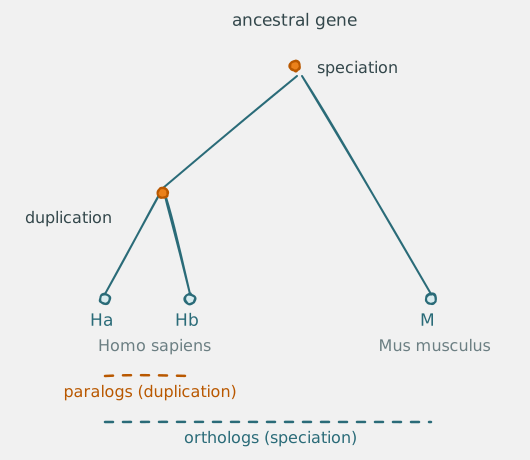
Genes in different species whose last shared event is speciation (orthologs).

Paralogy

Genes whose last shared event is a gene duplication (paralogs): a duplicated gene occupying a second position in the same genome.

Paralogs often keep similar functions; freed from the original selective pressure, one copy may mutate and acquire a new function.

Gene tree of an ancestral gene: a speciation event splits human and mouse lineages, and a later duplication inside the human lineage creates the paralogous pair Ha and Hb, while Ha (or Hb) and the mouse gene M are orthologs

Sequence similarity and ancestry

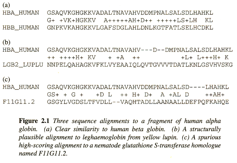
Alignment places residues into corresponding positions under a scoring model.
Identical residues can arise through common ancestry or by chance.
Statistically significant similarity can provide evidence for homology.

What can’t we see with sequence similarity?

$What can\'t we see with sequence similarity?$

Convergent Evolution

Sequence Alignment

Sequence alignment is:

A task of locating equivalent regions of two or more sequences to maximize their similarity

Sequence Alignment

Sequence Alignment: some notes

Better on AA or NN sequences?

Is easier to detect homology when comparing protein sequences than when comparing nucleic acid sequences.

1) Just 4 symbols in DNA, 20 in AA chain

Given the same sequence length,

AAs sequence provides with more information
Similarity by chance is much more probable in Nucleotide sequences (for the same sequence length).

Sequence Alignment: some notes

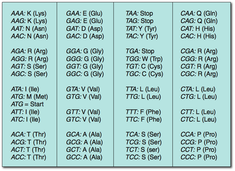
The Genetic Code is Redundant

There are two or more different codons for most amino acids.

Sequence Alignment: some notes

Dot Plots

Local and global similarity

Local similarity: similar regions within sequences that may differ elsewhere.

Global similarity: similarity across the full lengths of the sequences.

Why use a dot plot?

Visualise similarities without first choosing a local or global alignment.
Identify matching regions between two sequences.
Detect repeats within a sequence.

Global T F T T A L I L L A V A V

F - - T A L - L L A - A V

Local T F T T A L I L L - A V A V

- - F T A L - L L A A V - -

The same pair, aligned globally (upper rows: gaps added where the ends are forced together) and locally (lower rows: only the best-scoring stretch is kept, gaps at the trimmed ends).

Dot Plots

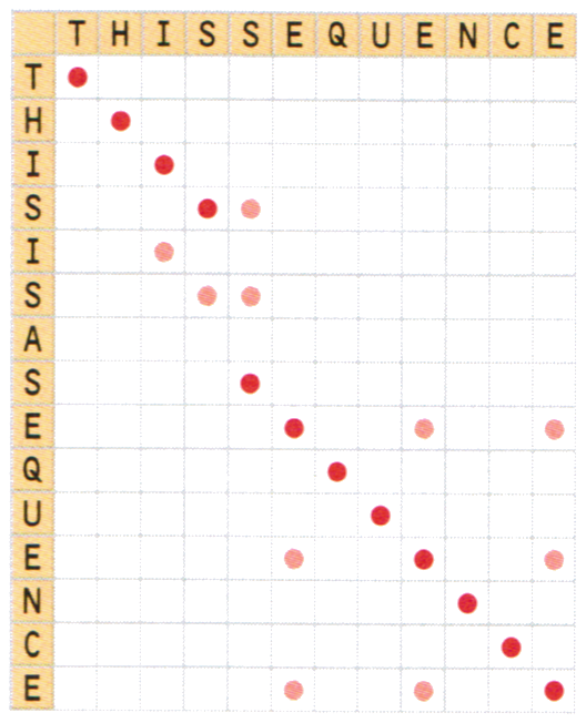
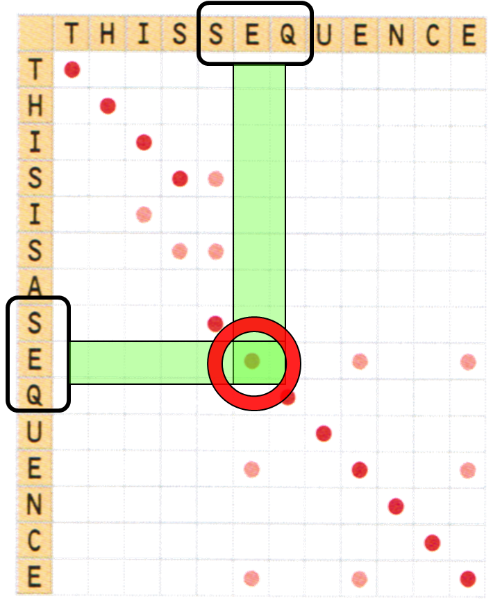
Dot plot of THISISASEQUENCE (vertical axis) against THISSEQUENCE (horizontal axis), raw single-residue matches

Raw single-residue matches: the diagonal shows through, but isolated chance dots bury the pattern. Sequences here: THISISASEQUENCE vs THISSEQUENCE.

Dot Plots

Dot plot with a three-residue window marking a confirmed SEQ/SEQ match

With a 3-residue window, matches are judged over whole windows: the SEQ / SEQ match is confirmed (green) and isolated dots no longer count.

Dot Plots

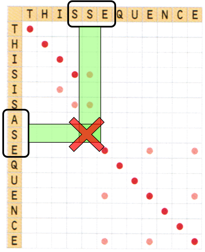
Dot plot with a three-residue window rejecting an SSE/ASE comparison (red cross)

The same rule rejects the wrong residues: SSE / ASE shares too little inside the window — no match.

Dot Plots

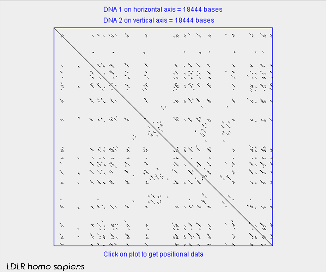
Self dot plot of the human LDL-receptor gene (18,444 bases): main diagonal plus many families of short off-diagonal repeats

The human LDL-receptor gene (18,444 bases) against itself: beyond the main diagonal, entire families of repeats populate the introns — the reality of whole-gene dot plots.

Dot Plots: Window Length

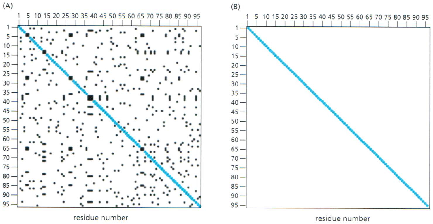
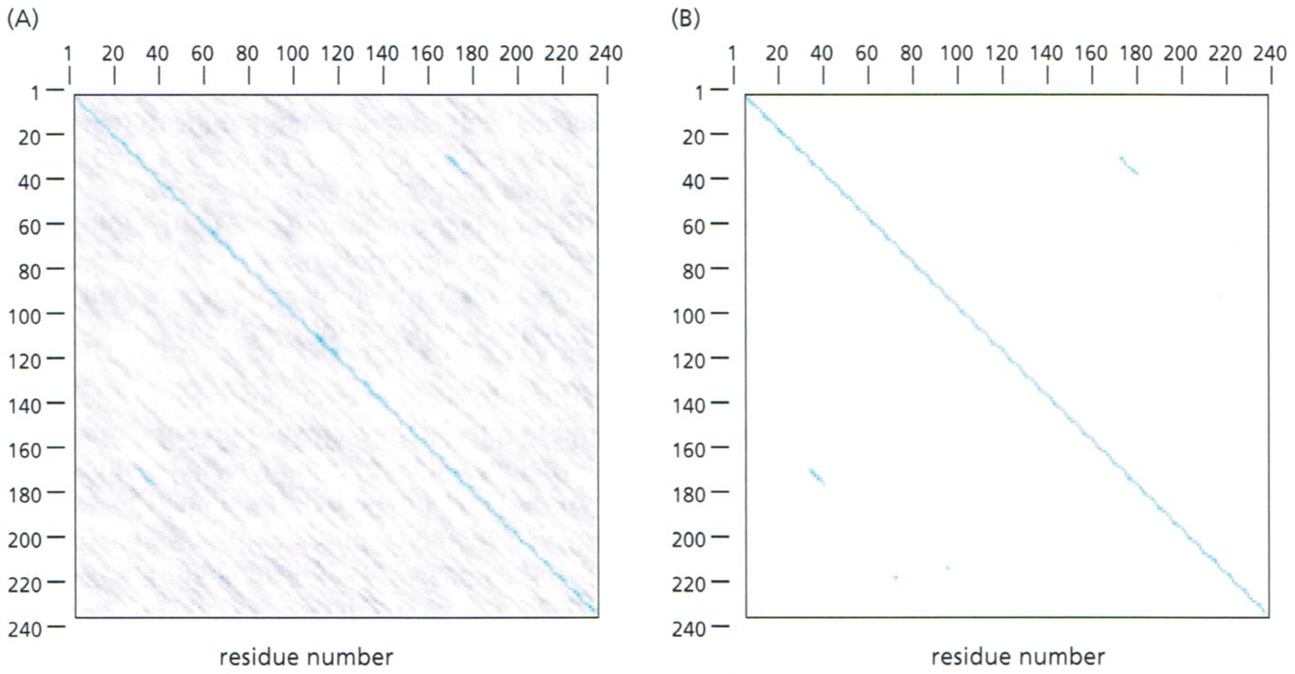
Self dot plots of a 95-residue sequence: raw matches (A) are noisy; window-filtered (B) keeps only the main diagonal

Self-comparison of a 95-residue sequence: single-residue matches (A) are mostly noise; a window filter with higher stringency (B) keeps the main diagonal alone.

Dot Plots: Window Length (SH2)

Self dot plots of a 240-residue SH2-containing protein: filtered version (B) reveals the main diagonal plus two short off-diagonal matches

A 240-residue SH2-containing protein: filtering reveals the main diagonal — plus two short off-diagonal matches (internal similarity).

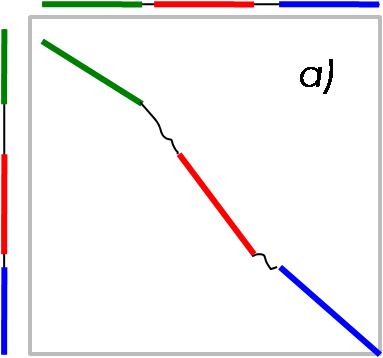
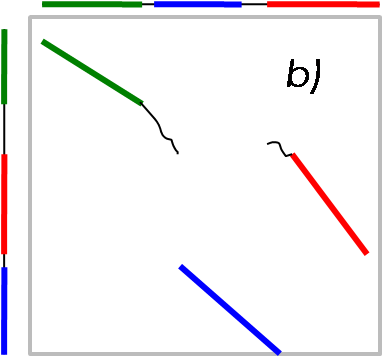
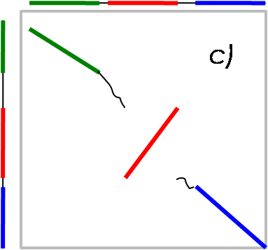
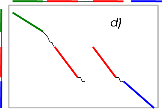
Dot plots: rearrangement patterns

Dot plot with a continuous diagonal

No rearrangement — one continuous diagonal

Dot plot with two segments aligning at unrelated offsets

Translocation — segments meet at unrelated offsets

Dot plot with an anti-parallel diagonal segment

Inversion — an anti-parallel (reversed) segment

Dot plot where one segment matches twice

Duplication — one segment matches twice

Amino acid Sequence Alignment

AA Sequence Alignment

Responds to the question whether any two sequences are related.

Four Main Steps

What sort of alignment should be considered?
What scoring system will rank alignments?
Which algorithm will seek good scoring alignments?
How do we assess the significance of an alignment score?

Alignment in AA sequences

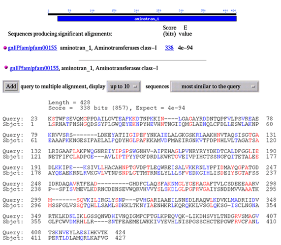
BLAST report for the aminotrans_1 query: a 338-bit match (E = 4e-94) against a Pfam class-I aminotransferase alignment

What the procedure can yield: a BLAST report with a 338-bit alignment (E = 4 × 10⁻⁹⁴) of the aminotrans_1 query to a Pfam class-I aminotransferase family.

Scoring homologous sequences

Homologous sequences can have different length.

Insertions, deletions, indels….. Marked as “-”

Scoring homologous sequences

On Statistical Significance

A simple alignment score

For an aligned pair of sequences, assign a score to each column:

Column	Score
Match	0
Mismatch	−1
Gap character	−G

The obvious strategy fails

Assume an alignment.
Score every column (table above).
Sum over all positions to get a score.
Repeat for all possible alignments — astronomically many, even for two moderately sized sequences.

There is a better way!

Dynamic programming reuses intermediate prefix scores instead of enumerating every alignment.

A Better Scoring

The total score is the sum of column terms for aligned pairs, plus gaps.

Identities and conservative substitutions

More likely in real alignments; positive scores.

Non-conservative changes

Less frequent in real alignments; negative scores.

Additive scoring

An Additive score system

Assumes mutations at different sites occurs independently.
This assumption is reasonable for DNA and proteins.
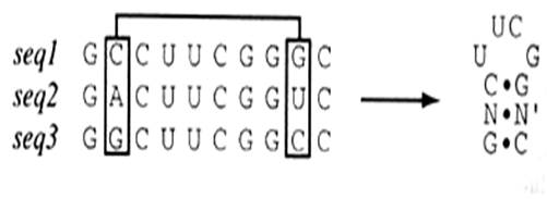
Could be not suitable for some RNA sequences.

Additive scoring

Probability models: first, the notation

position i	1	2	3	4	5	6
x	S	E	N	D	M	K
y	A	E	N	D	L	Q

Two aligned, gap-free sequences of equal length — the situation the models assume. The index $i$ counts alignment columns.

Each column is judged against two models

Highlighted column, $i = 4$ : $x_{4} =$ D and $y_{4} =$ D.

Chance (background) model: $q_{x_{4}} = q_{D}$ and $q_{y_{4}} = q_{D}$ are just background residue frequencies — $q_{D} \approx 5.4%$ across a protein database. The column’s chance probability is $q_{x_{4}} q_{y_{4}} = q_{D}^{2} \approx 0.3%$ .
Related (pair) model: $p_{x_{4} y_{4}} = p_{DD}$ = how often D sits opposite D inside conserved blocks — usually much more than 0.3%.

Same arithmetic for the mismatch column $i = 5$ : $q_{x_{5}} q_{y_{5}} = q_{M} q_{L} \approx 0.25%$ . The substitution score (next) compares related vs chance, column by column.

Sequence probability models

For aligned, ungapped sequences of equal length, let $q_{a}$ denote a background residue probability and $p_{ab}$ an aligned-pair probability.

Independent background model

$P (x, y ∣ R) = i \prod q_{x_{i}} q_{y_{i}}$

Aligned-pair model

$P (x, y ∣ M) = i \prod p_{x_{i} y_{i}}$

The models assume independence between alignment columns.

Log-odds alignment scores

The odds ratio compares the two models:

$\frac{P ( x , y ∣ M )}{P ( x , y ∣ R )} = i \prod \frac{p _{x_{i} y_{i}}}{q _{x_{i}} q _{y_{i}}} .$

Taking logarithms gives an additive score:

$s (a, b) = lo g \frac{p _{ab}}{q _{a} q _{b}}, S = i \sum s (x_{i}, y_{i}) .$

The logarithm base and scaling determine the score units.

Substitution matrices

$s (a, b)$ defines a matrix, known as score matrix or substitution matrix (SM).

A symmetric matrix for 20 amino acids has 210 distinct residue-pair entries, including the diagonal; gap penalties are separate.

Two main Substitution Matrices are usually employed:

PAM matrices model accepted point mutations.
BLOSUM, or BLOck SUbstitution Matrices, are built from gap-less conserved blocks.

Accepted point mutations (PAM)

Computed by Margaret Dayhoff in 1978 (also known as Dayhoff matrices): 1572 accepted point mutations in 71 families of closely related proteins.
PAM1 models an average of 1 accepted mutation per 100 residues; PAMn is PAM1 raised to the power n — PAM250 models strongly diverged sequences.
After many cycles a residue may mutate several times — even back to its original state — so PAM distance is not proportional to evolutionary time: families evolve at different rates.

BLOSUM, or BLOck SUbstitution Matrices

Henikoff and Henikoff, 1992: built from local alignments — the BLOCKS database of gap-less conserved blocks of protein families.
High numbers (BLOSUM80): closely related sequences; low numbers (BLOSUM45): more divergent ones.
BLOSUM62 is the de facto standard in protein database searches and sequence alignments.

PAM or BLOSUM?

	PAM (Dayhoff, 1978)	BLOSUM (Henikoff, 1992)
Built from	closely related families	gap-less conserved blocks
Alignment used	global	local
Numbering	higher = more diverged (PAM250)	higher = closer (BLOSUM80)
Typical choice	distant relatives	searches: 80, 62, 45

Match the matrix to the expected divergence: there is no universally correct matrix.

BLOSUM62: look up a residue-pair score

Reading BLOSUM62 scores

The score depends on which residues are aligned—not only whether they match.

Residue pair	BLOSUM62 score	Interpretation
W / W	+11	A tryptophan match
N / N	+6	An asparagine match
S / A	+1	A favourable non-identical pair
E / A	−1	An unfavourable pair
W / D	−4	A more strongly penalised pair

A substitution score is a log-odds score, not a mutation probability. Add the scores over aligned pairs; account for gaps separately.

Linear gap costs

For a gap of length $k$ , subtract the cost $d$ once per gap character:

$γ (k) = - k d, d > 0.$

Gap length	At $d = 8$	Contribution to the score
1	`−`	−8
2	`−−`	−16
3	`−−−`	−24

All worked examples in this section use BLOSUM62 and a linear gap cost of 8, unless you change it in the laboratory.

Affine gap costs

Opening one long gap can cost less than opening several short ones. Here $o$ is the opening cost and $e$ is the extension cost:

$γ (k) = - o - (k - 1) e, k \geq 1.$

With $o = 8$ and $e = 1$ :

Pattern	Calculation	Score contribution
One gap of length 3	$- 8 - 2 \times 1$	−10
Three separate gaps of length 1	$3 \times (- 8)$	−24

favoured — one long gap: $- 8 - 6 \times 1 =$ −14

ATGTAGTGTATAGTACATGCA

ATGTAG——-TACATGCA

penalised — three openings: $- 3 \times 8 - (1 + 1 + 2) \times 1 =$ −28

ATGTAGTGTATAGTACATGCA

ATGTA–G–TA—CATGCA

The simple recurrence we will use assumes linear costs. Affine costs require additional states, as in Gotoh’s algorithm.

Source: TIV-048 · Bioinformatica_Tema_IV.tex · line 878. Replaces the original screenshot-based treatment with editable, computed examples. Scoring data: BLOSUM62, distributed with Biopython (original matrix: Henikoff & Henikoff, 1992, https://www.pnas.org/doi/10.1073/pnas.89.22.10915). Algorithm reference: https://www.ncbi.nlm.nih.gov/books/NBK550342/. The examples use an explicitly chosen linear gap cost of 8, not BLAST’s default affine gap costs. Rows index y; columns index x. Tied optimal predecessors are retained; demonstrations follow diagonal, then up, then left when tied. Local endpoint ties use the first maximum in row-major order. The gap-length symbol is now consistently k. Some software uses −o−ke instead; always check the convention. Gotoh (1982): https://doi.org/10.1016/0022-2836(82)90398-9. The legacy verbatim DNA example (one long gap vs three separate openings) restored on 2026-10-21 as native monospace blocks; affine scores computed under o = 8, e = 1: single gap of length 7 → −8−6×1 = −14; gaps of 2, 2, 3 → −3×8−4×1 = −28.

Score an alignment, one column at a time

Column	1	2	3	4
x	S	E	N	D
y	A	−	N	D
Score	+1	−8	+6	+6

Total = 1 − 8 + 6 + 6 = 5.

This scores one proposed alignment. How do we find the best alignment without trying every possibility?

Dynamic programming: reuse prefix scores

A cell stores the best score for two prefixes of the sequences.

For example, $F (2, 3)$ aligns SEN with AN: the first three residues of $x$ and the first two of $y$ .

The last alignment column must contain a residue pair, a gap in $x$ , or a gap in $y$ . Each choice extends a smaller prefix alignment whose best score is already known.

Compute each cell once: $mn$ interior cells for lengths $m$ and $n$ . This gives $O (mn)$ time for the linear-gap model.

Needleman–Wunsch: align both complete sequences

Global alignment consumes every residue of both sequences, including their ends.

Stage	What to do
Initialise	Charge for aligning a prefix against an empty sequence.
Fill	Choose the best of three ways to enter each cell.
Trace back	Start at the bottom-right cell; stop at the origin.

The final score belongs to the bottom-right cell, even if another cell contains a larger value.

Global alignment: the recurrence

Rows consume $y_{i}$ ; columns consume $x_{j}$ . Let $F (i, j)$ be the best prefix-alignment score.

$F (i, j) = max ⎩ ⎨ ⎧ F (i - 1, j - 1) + s (x_{j}, y_{i}) F (i - 1, j) - d F (i, j - 1) - d align the two residues gap in x gap in y$

$F (0, 0) = 0, F (i, 0) = - i d, F (0, j) = - j d .$

Store every tied best predecessor. Several optimal alignments can share the same score.

Three moves, three alignment columns

Traceback move	Consume from x?	Consume from y?	Append this column
↖ Diagonal	Yes	Yes	residue / residue
↑ Up	No	Yes	`−` / residue
← Left	Yes	No	residue / `−`

Tracing backwards discovers the alignment from right to left. Reverse the collected columns to display it in sequence order.

The score table and the traceback path describe the same alignment. Its column scores must sum to the final cell score.

Our worked example: SEND and AND

x → S E N D

y ↓ A N D

These are short protein sequences, written with one-letter amino-acid codes.

Scoring matrix: BLOSUM62.
Linear gap cost: 8 per gap character.
A $4 \times 5$ score grid includes the empty-prefix row and column.

We will use these same inputs for global and local alignment.

Initialise the global grid

First cell: compare S with A

Second cell: a gap can be the best choice

Continue across the row, then down

Source: TIV-058 · Bioinformatica_Tema_IV.tex · line 1053. Replaces the original screenshot-based treatment with editable, computed examples. Scoring data: BLOSUM62, distributed with Biopython (original matrix: Henikoff & Henikoff, 1992, https://www.pnas.org/doi/10.1073/pnas.89.22.10915). Algorithm reference: https://www.ncbi.nlm.nih.gov/books/NBK550342/. The examples use an explicitly chosen linear gap cost of 8, not BLAST’s default affine gap costs. Rows index y; columns index x. Tied optimal predecessors are retained; demonstrations follow diagonal, then up, then left when tied. Local endpoint ties use the first maximum in row-major order. F(2,1) illustrates a tie: diagonal and up both score −7. All tied predecessor arrows are stored. Compute the next cell: N/N adds +6 to −7, giving −1.

Complete the global score grid

Trace back from the bottom-right cell

Recover the alignment and check its score

Ties mean more than one best route

A score cell can have two or three equally good predecessors.

For SEND / AND with BLOSUM62 and $d = 8$ , $F (2, 1)$ has a tie:

$max {- 8 + 1, 1 - 8, - 16 - 8} = - 7.$

Both diagonal and up are optimal ways to reach this cell.

A tie in a cell does not necessarily create multiple optimal complete alignments: the final traceback may never visit that cell.

The interactive grid shows every tied arrow. Its demonstration follows diagonal, then up, then left when tied.

Laboratory: change the gap cost

Source: TIV-063 · Bioinformatica_Tema_IV.tex · line 1153. Replaces the original screenshot-based treatment with editable, computed examples. Scoring data: BLOSUM62, distributed with Biopython (original matrix: Henikoff & Henikoff, 1992, https://www.pnas.org/doi/10.1073/pnas.89.22.10915). Algorithm reference: https://www.ncbi.nlm.nih.gov/books/NBK550342/. The examples use an explicitly chosen linear gap cost of 8, not BLAST’s default affine gap costs. Rows index y; columns index x. Tied optimal predecessors are retained; demonstrations follow diagonal, then up, then left when tied. Local endpoint ties use the first maximum in row-major order. First reproduce the global score 5 with gap cost 8. Then change the cost to 2 and recompute. Inputs accept 1–10 standard amino-acid letters; gaps in input are not allowed. Predict the result before filling the grid.

Local alignment: find the strongest matching region

Keep SEND / AND, BLOSUM62 and the gap cost of 8. Change only the alignment objective.

Global: Needleman–Wunsch	Local: Smith–Waterman
Align all residues	Align the best-scoring subsequences
`SEND` / `A−ND`	`ND` / `ND`
$1 - 8 + 6 + 6 = 5$	$6 + 6 = 12$

Local alignment can omit unfavourable flanking regions. It does not charge gaps for the omitted residues outside the selected subsequences.

Smith–Waterman: add a zero-score restart

The extra zero allows an alignment to start at the current position.

$F (i, j) = max ⎩ ⎨ ⎧ 0 F (i - 1, j - 1) + s (x_{j}, y_{i}) F (i - 1, j) - d F (i, j - 1) - d restart align the residues gap in x gap in y$

Initialise the first row and column to zero. Trace back from a highest-scoring cell anywhere and stop at zero.

Source: TIV-065 · Bioinformatica_Tema_IV.tex · line 1212. Replaces the original screenshot-based treatment with editable, computed examples. Scoring data: BLOSUM62, distributed with Biopython (original matrix: Henikoff & Henikoff, 1992, https://www.pnas.org/doi/10.1073/pnas.89.22.10915). Algorithm reference: https://www.ncbi.nlm.nih.gov/books/NBK550342/. The examples use an explicitly chosen linear gap cost of 8, not BLAST’s default affine gap costs. Rows index y; columns index x. Tied optimal predecessors are retained; demonstrations follow diagonal, then up, then left when tied. Local endpoint ties use the first maximum in row-major order. Smith & Waterman (1981): https://doi.org/10.1016/0022-2836(81)90087-5. If no cell is positive, the optimal local score is zero and there is no positive-scoring local alignment.

Local alignment: see the zero restart

Fill the local grid

Trace back to zero

Source: TIV-068 · Bioinformatica_Tema_IV.tex · line 1258. Replaces the original screenshot-based treatment with editable, computed examples. Scoring data: BLOSUM62, distributed with Biopython (original matrix: Henikoff & Henikoff, 1992, https://www.pnas.org/doi/10.1073/pnas.89.22.10915). Algorithm reference: https://www.ncbi.nlm.nih.gov/books/NBK550342/. The examples use an explicitly chosen linear gap cost of 8, not BLAST’s default affine gap costs. Rows index y; columns index x. Tied optimal predecessors are retained; demonstrations follow diagonal, then up, then left when tied. Local endpoint ties use the first maximum in row-major order. Click traceback twice: D/D then N/N. Stop at F(1,2)=0; do not continue to the grid origin. The selected substrings are x[3–4] and y[2–3], with 1-based inclusive coordinates.

A longer protein example: explore both objectives

Source: TIV-069 · Bioinformatica_Tema_IV.tex · line 1275. Replaces the original screenshot-based treatment with editable, computed examples. Scoring data: BLOSUM62, distributed with Biopython (original matrix: Henikoff & Henikoff, 1992, https://www.pnas.org/doi/10.1073/pnas.89.22.10915). Algorithm reference: https://www.ncbi.nlm.nih.gov/books/NBK550342/. The examples use an explicitly chosen linear gap cost of 8, not BLAST’s default affine gap costs. Rows index y; columns index x. Tied optimal predecessors are retained; demonstrations follow diagonal, then up, then left when tied. Local endpoint ties use the first maximum in row-major order. BLOSUM62, linear d=8: local score 20 for AWGHE/AW−HE; global score −8. The toy example is deliberately short. Changing the gap cost or matrix changes the optimisation problem. This replaces the old BLOSUM50 worked example and its screenshots.

Global versus local: predict before computing

Decision	Needleman–Wunsch	Smith–Waterman
First row and column	Accumulated gap costs	Zero
Candidate moves	Diagonal, up, left	Diagonal, up, left, zero
Traceback starts	Bottom-right cell	A highest-scoring cell
Traceback stops	Origin	A zero-score cell

Predict: for W versus D, BLOSUM62 gives −4 and the gap cost is 8. What does each algorithm return?

Global: score −4, alignment W / D. Local: score 0, no positive-scoring alignment.

A high score under a scoring model is not yet evidence of homology — quantify it first (next section).

Statistical significance of a local score

For sufficiently long random sequences and an appropriate scoring model, optimal local-alignment scores follow an extreme-value law:

$E = K m n e^{- λ S}$

$P = 1 - e^{- E} \approx E (small E)$

$m, n$ : sequence lengths; $S$ : alignment score.
$K, λ$ : calibrated by the scoring system and the residue background model — not from Smith–Waterman itself.

Illustrative E-values

With approximate BLOSUM62 constants $K = 0.13$ , $λ = 0.318$ , $m = 1000$ , $n = 100$ :

Score $S$	$E$ -value
40	3.9 × 10⁻²
50	1.6 × 10⁻³
60	6.7 × 10⁻⁵

Every +10 in score divides the expected count of chance matches by ≈ 24.

The $E$ -value is an expected count of chance matches, not the probability that an alignment is homologous.

Identity and similarity

Percent identity: identical residue pairs divided by the stated alignment-length denominator, multiplied by 100.
Percent similarity: residue pairs satisfying a specified similarity rule, often a positive substitution score, divided by the stated denominator.
State whether gaps are included and which scoring matrix defines similarity.

Worked example — SEND / A−ND: 3 identical residue pairs. Over all 4 alignment columns: 75% identity. Excluding the gap column: 100% of residue–residue columns. The denominator changes the number.

These percentages describe an alignment. Homology describes common ancestry.

BLAST

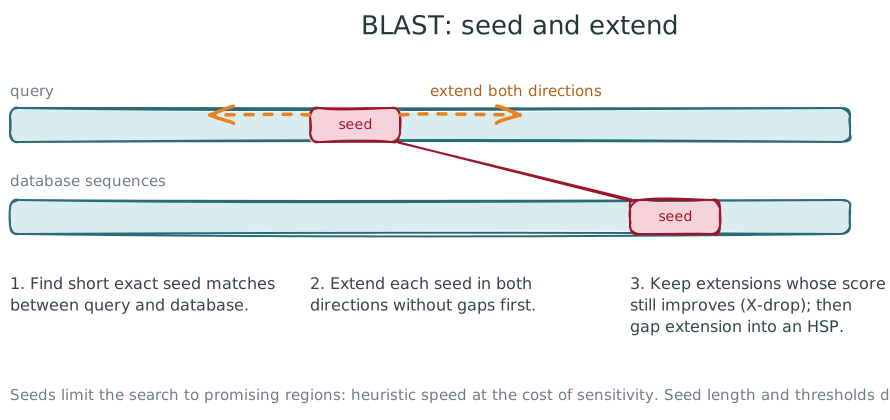
Heuristic search: seed and extend

BLAST — Altschul et al., 1990.
Finds short exact seed matches, extends them in both directions while the score improves, and keeps high-scoring segment pairs (HSPs) with bit scores and $E$ -values.

Why not full dynamic programming?

Smith–Waterman needs $O (nm)$ cells: a 1 000-residue query against a 10⁸-residue database ≈ 10¹¹ updates — infeasible.
Seeding limits the work to each seed’s neighbourhood, trading some sensitivity.

Query and database bars with a highlighted seed match connected by a line; dashed orange arrows show extension in both directions; three numbered steps explain seed finding, extension and HSP formation. — BLAST finds short exact seed matches between query and database, then extends them in both directions while the score keeps improving.

FASTA

Pearson and Lipman, 1988: heuristic local alignment.
Uses a lookup table of short words (ktup: 2 for proteins, 6 for DNA by default) to find dense diagonals of similarity.
Rebuilds the top diagonals with gap-aware, optimized local alignment.
Higher ktup: faster, less sensitive; lower ktup: slower, more sensitive.
https://fasta.bioch.virginia.edu/ (redirects to HTTPS; verified 2026-10-01)

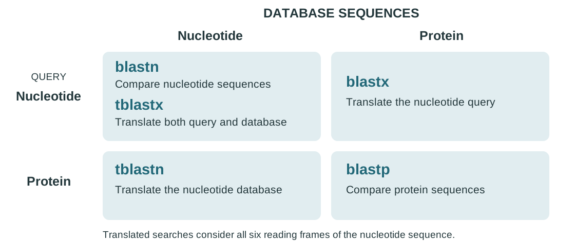
Choosing a sequence-search program

BLAST program selection by nucleotide or protein query and database

Multiple Alignment

Multiple Sequence Alignment

To align three or more biological sequences

We could think in an extension of dynamic programming methods for $N$ individual sequences:

Involves the construction of an $N$ -way or $N$ -dimensional equivalent of the $F$ matrix in a similar way than pairwise sequence alignment.
Not as computational efficient with large $N$ . Combinatorial explosion as the number of sequences increases!!!
Methods have been published to reduce the search space of the algorithm.
Dynamic programming is used with limitations on MSA.

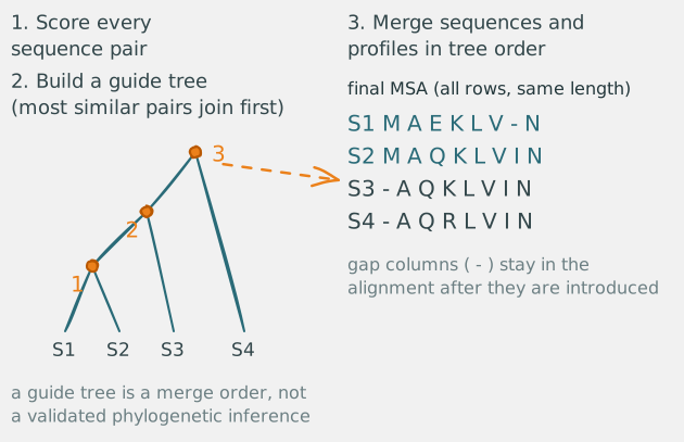
Progressive multiple alignment

Compute pairwise similarities or distances.
Build a guide tree or another ordering of the sequences.
Align sequences and profiles progressively in that order.
Early alignment errors can influence later steps.

A guide tree organises alignment; it is not automatically a validated phylogenetic inference.

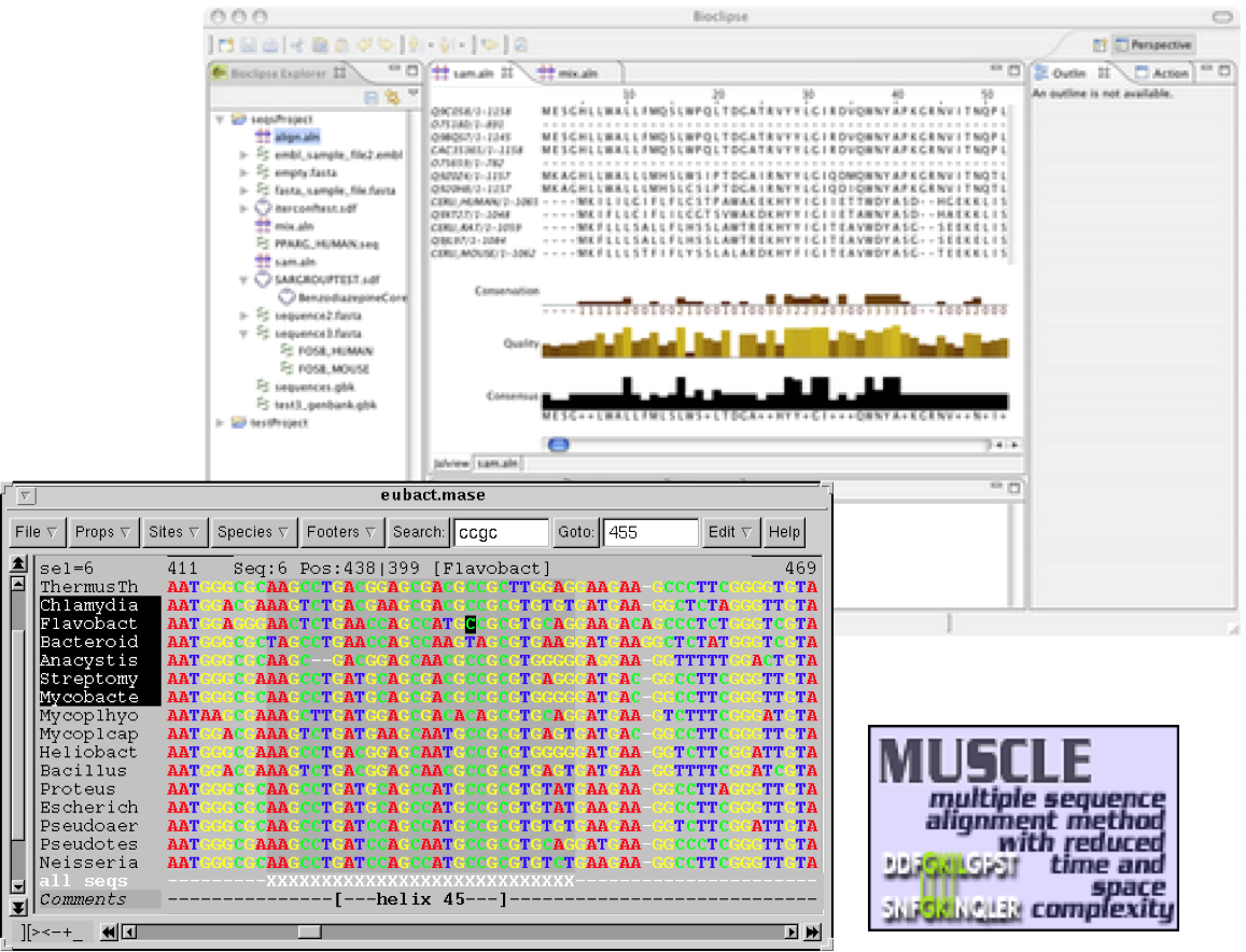
All pairwise scoring, a guide tree in which S1 and S2 merge first, then S3, then S4, and the final fixed-length multiple alignment with gap columns

Multiple sequence alignment software

Alignment programs

MUSCLE, Clustal Omega, MAFFT
Kalign and T-Coffee

Viewers and editors

Jalview
SeaView

The screenshot illustrates the original course software comparison. Its entries and interfaces are historical.

MSA software

The End

Sequence analysis

Motivation

Contents

Motivation

Sequence Analysis

Per-Sequence Analysis

Between Sequences

Profiles

Amino acid Features

Argos

Sequence profiles

Features on individual amino acids play some role in protein early secondary structure formation

Hydrophobicity scales

Hydrophobicity

Kyte-Doolittle

Hopp-Woods

Hydrophobicity: the two scales side by side

Hydrophobicity Profiles

Pairwise alignment

Evolution suggests

Comparing two sequences

Why is it useful?

Phylogenetic Tree of Life

Homology, orthology and paralogy

Homology

Orthology

Paralogy

Sequence similarity and ancestry

What can’t we see with sequence similarity?

Sequence Alignment

Sequence alignment is:

Sequence Alignment: some notes

Better on AA or NN sequences?

1) Just 4 symbols in DNA, 20 in AA chain

Sequence Alignment: some notes

The Genetic Code is Redundant

Dot Plots

Local and global similarity

Why use a dot plot?

Dot Plots

Dot Plots

Dot Plots

Dot Plots

Dot Plots: Window Length

Dot Plots: Window Length (SH2)

Dot plots: rearrangement patterns

Amino acid Sequence Alignment

AA Sequence Alignment

Four Main Steps

Alignment in AA sequences

Scoring homologous sequences

Homologous sequences can have different length.

On Statistical Significance

A simple alignment score

The obvious strategy fails

There is a better way!

A Better Scoring

Identities and conservative substitutions

Non-conservative changes

Additive scoring

An Additive score system

Probability models: first, the notation

Each column is judged against two models

Sequence probability models

Independent background model

Aligned-pair model

Log-odds alignment scores

Substitution matrices

Accepted point mutations (PAM)

BLOSUM, or BLOck SUbstitution Matrices

PAM or BLOSUM?

BLOSUM62: look up a residue-pair score

Reading BLOSUM62 scores

Linear gap costs

Affine gap costs

Score an alignment, one column at a time

Dynamic programming: reuse prefix scores

Needleman–Wunsch: align both complete sequences

Global alignment: the recurrence

Three moves, three alignment columns