The Human Genome Project and genome-wide association

From a genome sequence to a disease association

1 · Build a reference 2 · Describe variation 3 · Model populations 4 · Explain trait variation 5 · Test association 6 · Interpret responsibly

By the end, you should be able to calculate allele frequencies, distinguish heritability measures, choose a genotype model and explain why a GWAS hit is not automatically causal.

The Human Genome Project: what was achieved?

Milestone	Contribution
1990	International public project launched
2001	Draft human genome analyses published
2003	Project completed: high-quality reference, with gaps remaining

A shared coordinate system made it possible to connect sequence, genes, variation and phenotype. The reference was assembled from multiple donors; it was never a complete catalogue of human diversity.

NHGRI: Human Genome Project.

After the reference: variation and biological function

Project · landmark	Question	Contribution
HapMap · launched 2002	Which variants travel together?	Common SNPs and haplotypes; a foundation for GWAS
1000 Genomes / IGSR · Phase 3, 2015	Which variants occur across populations?	2,504 people, 26 populations; reference panels for variation and imputation
ENCODE · launched 2003	Where are candidate functional elements?	Maps of transcription, chromatin and gene regulation across cell types

Reference sequence → variation catalogue → biological interpretation.

Project names link to official resources. 1000 Genomes resource paper · ENCODE overview.

The 100,000 Genomes Project: bringing sequencing to patients

A clinical programme

Announced in 2012; Genomics England established in 2013.
100,000 genomes milestone reached in December 2018.
NHS participants affected by rare disease or cancer, with family members included.

What sequencing helps resolve

Rare disease: compare relatives to identify inherited or new variants.
Cancer: compare tumour and normal DNA to identify acquired variants.
Helped establish the NHS Genomic Medicine Service.

100,000 genomes ≠ 100,000 people: one person can contribute tumour and normal samples.

Project website: Genomics England · 2018 milestone and NHS legacy.

From clinical sequencing to population-scale health research

Project	Scale · dated milestone	Research purpose
UK Biobank	Whole genomes from ~500,000 participants, released in 2023	Link genetic variation to health records, lifestyle, imaging and disease outcomes
All of Us · United States	>414,000 short-read genomes in the Research Hub FAQ, checked September 2026	Study health and disease in a diverse cohort with linked health information

More participants improve statistical power. Diverse recruitment and good phenotype data determine which questions we can answer.

UK Biobank: 500k release · All of Us: available genomic data. Individual-level data require authorised research access.

Completion and diversity are different goals

Milestone	What it adds	What it does not mean
T2T-CHM13, 2022	Gapless autosomes and X in this assembly	Every human genome, or a Y chromosome
Complete Y, 2023	A resolved Y chromosome sequence	All Y-chromosome diversity
Draft pangenome, 2023	47 phased diploid assemblies	Exhaustive representation of humanity

Later work includes HPRC Release II (2025). These are dated landmarks, not a latest-release inventory. Completeness and population representation remain distinct goals.

Nurk et al. (2022) · Rhie et al. (2023) · Liao et al. (2023).

A reference is a coordinate system, not a “normal person”

A variant is described relative to a reference sequence.
Reference allele ≠ most frequent allele ≠ ancestral allele ≠ harmless allele.
Record the assembly, chromosome, position and alleles; for transcripts, include accession and version.
Different reference choices can change coordinates and variant representation.

Do not combine datasets until their builds and allele orientations have been checked.

HGVS: reference sequences.

Comparing genomes: always define the denominator

“Percent identical” depends on what is aligned and which differences count.

Comparison	Questions to ask
Two human genomes	SNPs only, or also indels and structural variants?
Human and another species	Orthologous aligned sequence, genes, or whole genomes?
Gene counts	Which annotation release and gene definition?

The source slide’s single percentages and fixed gene counts hid these choices. Genome similarity is not a ranking of biological complexity.

Karyotype: an ordered view of chromosomes

An ideogram

NHGRI Talking Glossary schematic of the 23 chromosome pairs: 22 numbered autosomal pairs, then X Y or X X Pairs ordered by size and banding; the 23rd pair is XX or XY.

A metaphase spread

NHGRI G-banded human male karyotype: photographed chromosomes of one cell classified and arranged in pairs Chromosomes are photographed and classified.

Figures: National Human Genome Research Institute — public domain (credit “National Human Genome Research Institute”); G-banded karyogram via Wikimedia Commons.

Chromosomes organise and package DNA

NHGRI schematic of DNA packaging into chromatin and a chromosome

Keep three terms separate

Homologues: maternal and paternal versions of a chromosome.
Sister chromatids: replicated copies of one chromosome.
Centromere: region that supports chromosome segregation.

An X-shaped chromosome is replicated; not every chromosome looks like an X.

Figure: NIH/NHGRI.

The vocabulary of genetic variation

Term	Meaning
Locus	A genomic position or region
Allele	One sequence version at a locus
Genotype	Allele combination carried by an individual
Haplotype	Alleles on the same physical chromosome copy
Allele frequency	Fraction of sampled chromosome copies carrying an allele
Prevalence	Fraction of people with a specified condition at a specified time

Diploid autosomal examples have two copies per person. Ploidy can differ elsewhere.

Allele frequency is counted from chromosome copies

In 100 diploid people, observe 49 AA, 42 Aa and 9 aa.

$p = f (A) = \frac{2 ( 49 ) + 42}{2 ( 100 )} = 0.70, q = f (a) = 0.30.$

Quantity	Value
Frequency of allele a	30% of chromosome copies
Frequency of genotype Aa	42% of people
People carrying at least one a	51% of people

These are three different quantities. Counting alleles does not require Hardy–Weinberg equilibrium.

Hardy–Weinberg: from allele frequencies to genotypes

For two alleles, $p + q = 1$ .

Random union of gametes gives:

$f (AA) = p^{2}, f (A a) = 2 pq, f (aa) = q^{2} .$

At $p = 0.7$ : 49%, 42%, 9%.

This is an expected distribution, not a claim that every population satisfies it.

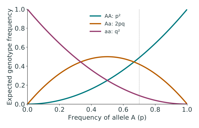
Expected AA, Aa and aa frequencies across allele frequency p

Figure: original plot of Hardy–Weinberg equations.

When Hardy–Weinberg expectations fail

Possible reason	Interpretation
Genotyping error	A technical problem to investigate
Population mixture or inbreeding	Genotype proportions may depart from random mating
Selection or disease ascertainment	Particular genotypes may be overrepresented
Sampling variation	A test can reject by chance

For case–control GWAS, HWE filtering is often assessed in controls. Choose thresholds for the study; do not treat every departure as an error.

PLINK: Hardy–Weinberg tests and filters.

Common disease can involve common and rare variants

The common disease–common variant hypothesis motivated early GWAS.

Many common variants have small marginal effects.
Rare variants can have large or small effects.
A common disease can contain monogenic subtypes and a polygenic majority.
Frequency and effect size do not determine each other by a universal rule.

Frequency, effect size and penetrance describe different properties.

Allele frequency and effect size shape discovery

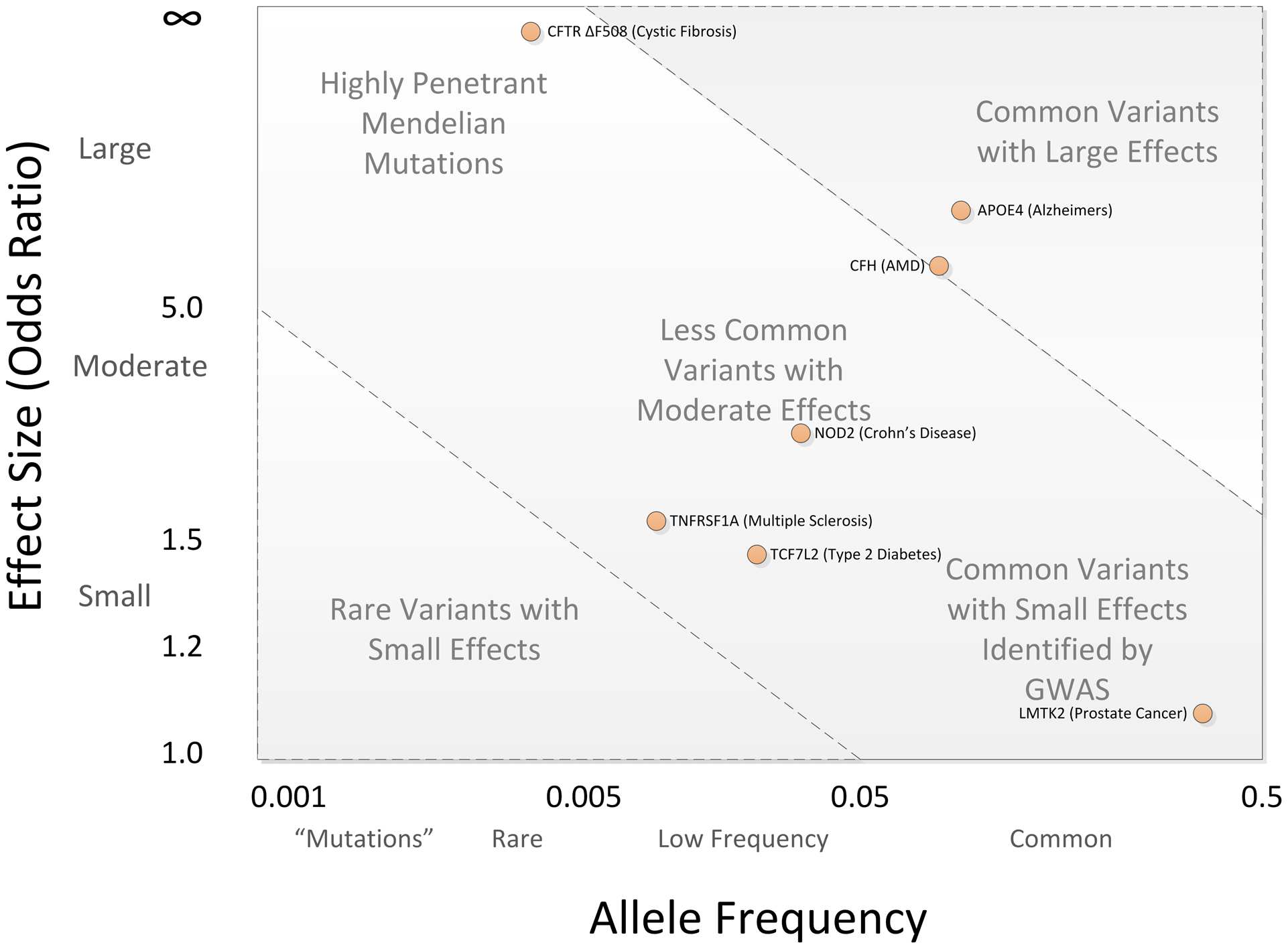
Published conceptual map of allele frequency against genetic effect size

Read this as a conceptual map

Rare, large-effect variants: family studies and sequencing can be informative.
Common, small-effect variants: large association studies are often needed.
Low frequency and small effect: especially difficult to detect.

Figure: Bush & Moore (2012), PLOS Computational Biology.

What genome sequencing enables

Locate and annotate genes and regulatory elements.
Identify variants in Mendelian disease and complex-trait studies.
Compare species and investigate evolutionary history.
Design molecular assays and gene-editing experiments.
Study gene expression, drug response and tumour evolution.

Sequence is a starting point: functional interpretation requires biological and clinical evidence.

Genetic architecture: four ideas that can coexist

How many loci?

Monogenic: one locus has a major role in a disorder.

Polygenic: many loci contribute to trait variation.

How do effects relate?

Pleiotropy: one genetic factor affects multiple traits.

Epistasis: the effect at one locus depends on genotype at another.

Monogenic disease does not mean identical outcomes

Example	Key gene(s)	Important qualification
Cystic fibrosis	CFTR, chromosome 7	Usually recessive; alleles and modifiers affect severity
Familial hypercholesterolaemia	Often LDLR, chromosome 19	APOB, PCSK9 and other mechanisms also occur

Penetrance, expressivity, environment and other genes can modify a monogenic condition.

NCBI: LDLR · NCBI: CFTR.

Polygenic inheritance: many contributions

Many variants+Environment→Variation in a trait

Each locus can follow Mendelian transmission while the overall trait is complex.
Height is quantitative; disease can be recorded as binary despite an underlying continuous liability.
A bell-shaped trait distribution is a useful model in some settings, not a necessary consequence of “many genes”.

Pleiotropy: one genetic change, several consequences

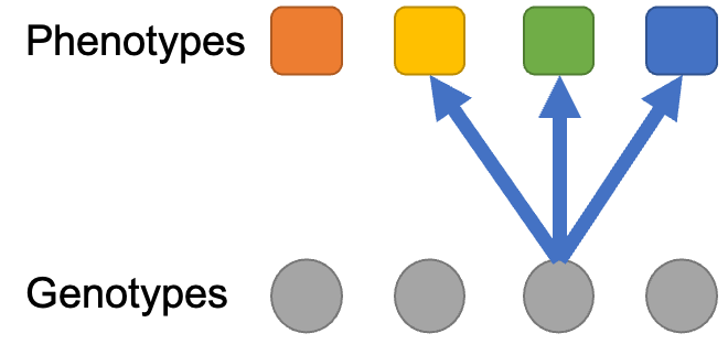
Source schematic with one genetic factor pointing to multiple phenotypes

Example: haemoglobin S

A change in HBB can contribute to red-cell sickling, anaemia and downstream organ complications.

Multiple clinical consequences may share one upstream mechanism.

Statistical association with several traits can also reflect LD or mediated effects.

Figure: supplied lecture. Sickle cell disease, GeneReviews.

Epistasis: an effect depends on another locus

An interaction model can include:

$Y = β_{0} + β_{1} G_{1} + β_{2} G_{2} + γ G_{1} G_{2} + ε .$

$γ \neq = 0$ means departure from additivity on this model’s scale.
Biological pathway interaction and statistical interaction are not identical.
Interaction estimates need adequate sample sizes and careful multiple-testing control.

A pathway can involve interacting proteins even when an additive statistical model predicts well.

Heritability describes variation in a population

$H^{2} = \frac{V _{G}}{V _{P}} and h^{2} = \frac{V _{A}}{V _{P}} .$

Measure	Numerator
Broad-sense $H^{2}$	Total genetic variance $V_{G}$
Narrow-sense $h^{2}$	Additive genetic variance $V_{A}$

Both use phenotypic variance in the denominator. Neither is the proportion of one person’s phenotype “caused by genes”.

Variance decomposition needs assumptions

Under a simplified model with uncorrelated components:

$P = μ + A + D + I + E, V_{P} = V_{A} + V_{D} + V_{I} + V_{E} .$

$A$ : additive genetic effects; $D$ : dominance; $I$ : epistasis; $E$ : residual environment and measurement.
Correlations among components add covariance terms.
Gene–environment interaction needs an explicit term; it cannot be added to the phenotype model and then omitted from its variance.

High heritability does not mean that an intervention cannot change the trait.

Yang et al. (2017): interpreting SNP heritability.

Kinship and relatedness are not the same coefficient

Pair, assuming no inbreeding	Kinship $ϕ$	Additive relationship $r = 2 ϕ$
Individual with self	1/2	1
Parent–child or full siblings	1/4	1/2
Grandparent–grandchild; half siblings	1/8	1/4
Aunt/uncle–niece/nephew	1/8	1/4
First cousins	1/16	1/8

Kinship is the probability that two sampled alleles are identical by descent. Shared environment and nonadditive effects prevent a general rule $h^{2} = correlation / r$ .

Association asks whether genotype and phenotype co-vary

A GWAS tests genetic variants across the genome for association with a phenotype.

A signal can arise from a causal variant, a correlated marker in LD, population structure, batch effects or chance.

A small p-value is evidence against a model’s null hypothesis—not proof of a causal gene or a large effect.

WTCCC (2007): a landmark multi-disease GWAS.

Study designs: binary, quantitative and molecular traits

Phenotype	Example	Common starting model
Binary outcome	Cases versus controls	Logistic regression
Quantitative trait	Height, blood lipid concentration	Linear regression
Molecular trait	Gene expression or protein abundance	QTL model appropriate to the measurement

Case–control sampling does not directly estimate population disease prevalence. An eQTL is associated with expression; it is not automatically a disease mechanism.

PLINK 2 association models.

A GWAS workflow students can follow

1 · Define phenotype and sampling2 · Genotype / sequence + quality control3 · Align alleles, phase and impute4 · Fit association models + covariates5 · Check calibration + replicate6 · Fine-map and investigate function

Document genome build, allele coding, ancestry composition, sample overlap and each exclusion step. These choices are part of the analysis, not housekeeping.

Quality control protects the association test

Samples	Variants
Missingness and contamination	Call rate and batch differences
Duplicates and relatedness	Allele alignment and strand ambiguity
Phenotype and covariate consistency	Allele counts/frequency
Population structure	HWE in an appropriate comparison group
Consent and permitted use	Imputation quality

Thresholds depend on study design and data quality. Rare-variant tests require special attention to low counts.

PLINK 2 filtering documentation.

Imputation predicts unobserved genotypes

Observed markers+Reference haplotypes→Genotype probabilities

Phasing estimates which alleles share a chromosome copy.
Imputation uses shared haplotype patterns to infer untyped variants.
Dosage is an expected allele count between 0 and 2, not always an integer.
Reference-panel match, allele frequency and local LD affect accuracy.

Use imputation quality and uncertainty in downstream analysis.

Quantitative-trait GWAS: one SNP plus covariates

$Y_{i} = β_{0} + β_{G} G_{i} + γ^{T} C_{i} + ε_{i} .$

$G_{i}$ : 0, 1 or 2 copies of the chosen effect allele, or imputed dosage.
$C_{i}$ : covariates such as age, study batch and ancestry components.
$β_{G}$ : mean trait change per additional effect allele under the additive model.
Test $H_{0} : β_{G} = 0$ ; report effect estimate, uncertainty and effect allele.

Changing which allele is counted reverses the sign of the estimated effect.

PLINK 2: linear and logistic regression.

Binary-trait GWAS: log odds, not the phenotype itself

$lo g \frac{Pr ( Y _{i} = 1 )}{1 - Pr ( Y _{i} = 1 )} = β_{0} + β_{G} G_{i} + γ^{T} C_{i} .$

$Odds ratio per allele = e^{β_{G}} .$

An odds ratio is not an absolute risk and is not generally a risk ratio. Baseline risk and ascertainment matter. Very low allele counts or separation may require Firth or other suitable methods.

PLINK 2 association documentation.

Genotype coding defines the question

Model for allele a	AA	Aa	aa	SNP degrees of freedom
Additive dosage	0	1	2	1
Dominant	0	1	1	1
Recessive	0	0	1	1
Genotypic	baseline	indicator 1	indicator 2	2

“Dominant” and “recessive” here describe a fitted contrast for a chosen allele; they are not established modes of disease inheritance.

Four genotype models, four patterns

Four plots show additive, dominant, recessive and unconstrained genotypic mean patterns

Compare the mean at Aa with the means at AA and aa. Curves are illustrative, not patient results.

Figure: original schematic plots; axes and allele coding explicitly labelled.

A two-degree-of-freedom test allows a separate heterozygote effect

$Y_{i} = β_{0} + β_{1} 1 (G_{i} = 1) + β_{2} 1 (G_{i} = 2) + γ^{T} C_{i} + ε_{i} .$

Joint null: $H_{0} : β_{1} = β_{2} = 0$ .

No requirement that the heterozygote mean lies halfway between homozygotes.
More flexibility, but usually less power than a correctly specified one-df model.
For a binary trait, apply this linear predictor to the logit, not directly to a 0/1 response.

Why genome-wide significance is stringent

One million tests at a nominal $p < 0.05$ would yield about 50,000 false positives under the global null.

$α_{Bonferroni} = \frac{0.05}{1 0 ^{6}} = 5 \times 1 0^{- 8} .$

This is a conventional common-variant GWAS benchmark. LD makes tests correlated; sequencing, ancestry, variant sets and multiple phenotypes can require different corrections.

A discovery still needs replication and a credible analysis.

Reading a Manhattan plot

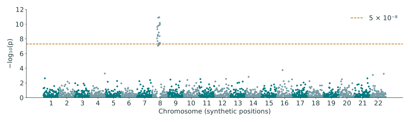
Synthetic Manhattan plot with chromosome position, minus log10 p-values and a 5e-8 threshold

Each dot is a variant. A cluster can reflect many correlated markers tagging one signal.

Figure: reproducible synthetic data, generated for teaching; not a real disease GWAS.

Population structure can mimic genetic association

Suppose ancestry groups differ in allele frequency and disease prevalence for environmental or sampling reasons.

A pooled genotype–disease association can then appear without a causal allele effect.

Inspect ancestry structure, phenotype distribution and study batches.
Include appropriate covariates and consider mixed models.
Genetic ancestry is a statistical description, not a substitute for social or environmental variables.

Price et al. (2006).

Relatedness is a separate modelling problem

Relatives share alleles across the genome, so their residuals may be correlated.

$Y = X β + u + ε, u \sim N (0, σ_{g}^{2} K) .$

$K$ represents genetic similarity. Mixed models can account for relatedness and sample structure; binary outcomes need appropriate extensions.

Family-based designs can also be deliberately used for robust within-family inference. They are not inherently flawed GWAS designs.

Kang et al. (2010).

Linkage disequilibrium is correlation across loci

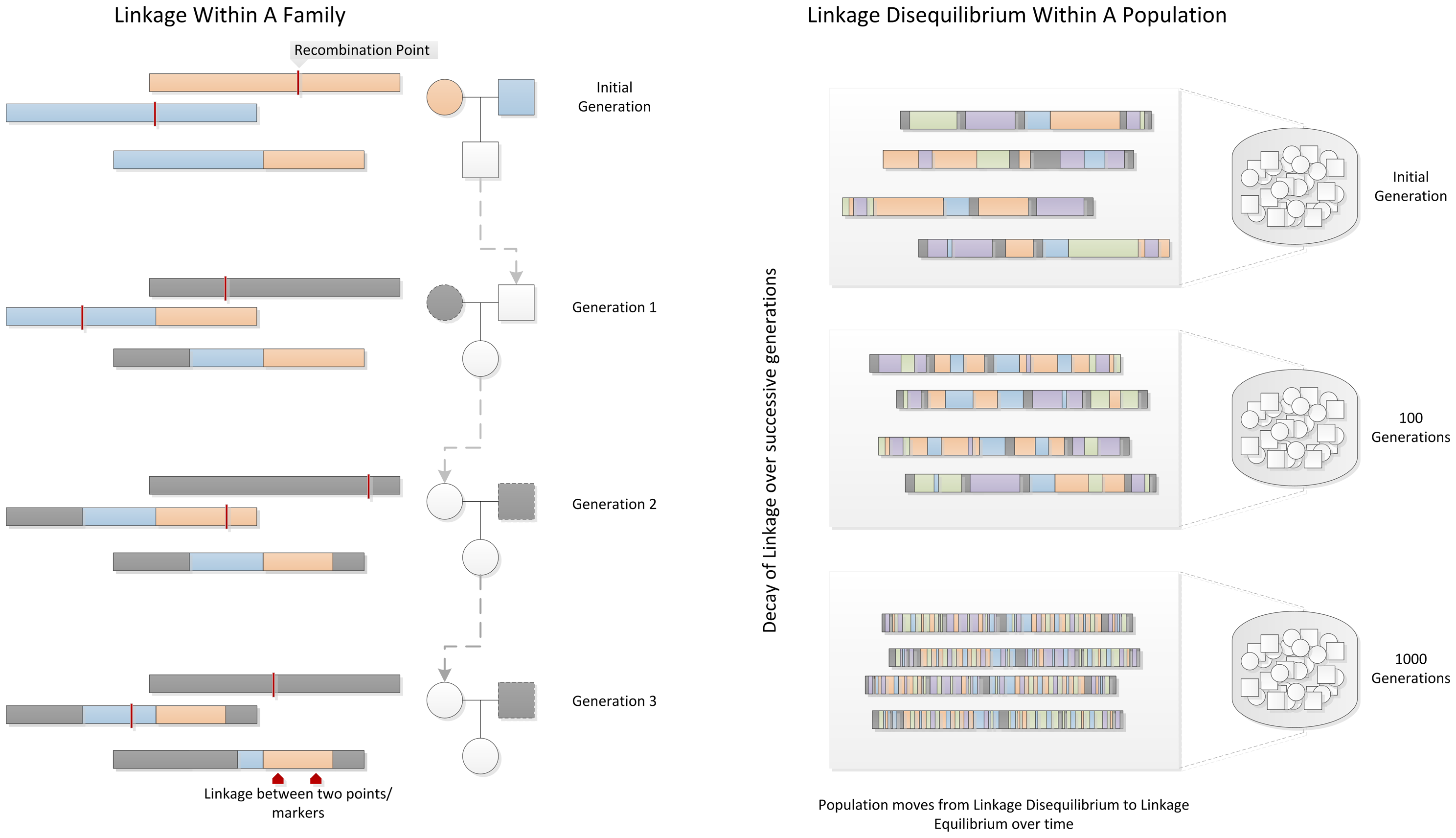
Published comparison of linkage within families and linkage disequilibrium in populations

Distinguish the concepts

Linkage: nearby loci tend to cosegregate in families.

LD: alleles at different loci occur together non-randomly in a population.

Recombination, demography and selection shape LD.

Figure: Bush & Moore (2012), PLOS Computational Biology.

A genotyped marker can tag an unobserved causal variant

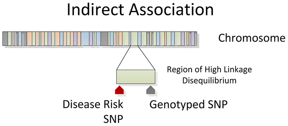
Published schematic showing indirect association through linkage disequilibrium

A hit identifies a region to investigate

A lead SNP can be a proxy.
LD patterns differ between populations.
The closest gene is not automatically causal.
Fine-mapping and functional evidence help distinguish alternatives.

Figure: Bush & Moore (2012), PLOS Computational Biology.

A small numerical example of LD

For alleles A and B at two loci:

$D = f (A B) - p_{A} p_{B}, r^{2} = \frac{D ^{2}}{p _{A} ( 1 - p _{A} ) p _{B} ( 1 - p _{B} )} .$

If $p_{A} = p_{B} = 0.5$ and $f (A B) = 0.4$ , then $D = 0.15$ and $r^{2} = 0.36$ .

If haplotypes AB and ab each have frequency 0.5, $r^{2} = 1$ : perfect tagging in that population. If the loci are independent, $D = 0$ .

Discovery and prediction use different strategies

Single-variant GWAS usually tests one marker at a time, adjusting for covariates.

A joint predictive model instead combines many markers:

$Y = β_{0} + j = 1 \sum m β_{j} G_{j} .$

There are $2^{m}$ possible subsets of $m$ markers. Exhaustive subset search quickly becomes infeasible; LD also makes coefficients difficult to estimate without suitable constraints.

Pairwise interactions grow quadratically

For distinct unordered pairs among $m$ markers:

$Number of pairs = (2 m) = \frac{m ( m - 1 )}{2} .$

For $m = 1, 000$ , this gives 499,500 interaction terms, in addition to main effects.

Use $\sum_{j < k} γ_{jk} G_{j} G_{k}$ to count each pair once. The source expression $m! / (m - 2)!$ counted each pair twice.

Predictive modelling: fit, tune, then evaluate

Approach	Main idea
Ridge / Bayesian shrinkage	Stabilise many small, correlated effects
LASSO / elastic net	Shrink coefficients, possibly selecting a subset
Trees, boosting, neural networks	Model flexible patterns; need careful validation
Biological priors / pathway models	Use external knowledge without assuming it proves causality

Keep relatives and overlapping samples from leaking across evaluation splits. Tune in training data; report performance in independent data.

Polygenic scores are not individual destinies

$PGS_{i} = j \sum β_{j} G_{ij} .$

Score performance depends on discovery sample size, LD, ancestry, phenotype and environment.
Evaluate discrimination and calibration in the intended population.
A score is not an absolute risk without an appropriate risk model.
Clinical benefit and fairness require evidence beyond association significance.

Martin et al. (2019).

“Missing heritability”: which gap are we discussing?

Quantity	What contributes?
Significant-hit variance explained	Variants that pass a chosen discovery threshold
SNP-based heritability	Additive effects tagged by the analysed variant set
Pedigree-based estimate	Familial resemblance under a specified model

These need not agree. Many effects are too small to pass single-variant significance, even when their combined contribution can be estimated.

Yang et al. (2017).

Why estimates and prediction can differ

Rare or structural variants may be poorly tagged by the analysed markers.
Many weak associations lie below the discovery threshold.
Phenotype noise and environmental differences change what is estimated.
Family models can be affected by shared environment and their assumptions.
Nonadditive effects and gene–environment interactions can matter, depending on the trait.

Do not label all unexplained variance “missing genetic effects”.

From a GWAS hit to a biological explanation

Association→Fine-mapping→Gene / tissue hypothesis→Functional tests

Replication checks whether the association survives another sample. Colocalisation can test whether two signals may share a causal variant. Experiments can test a proposed mechanism.

Each step adds evidence; none should be silently replaced by “nearest gene”.

The central ideas to take away

Reference genomes provide coordinates; human variation is broader than one reference.
Allele frequency, genotype frequency and prevalence are different quantities.
Heritability is a population-specific variance ratio.
GWAS tests association; LD and confounding shape its signals.
Good inference needs quality control, appropriate models, replication and honest uncertainty.

Key readings and teaching sources

Questions

A question mark — questions and discussion