Bioinformatics · Universitat Politècnica de Catalunya
Alexandre Perera-Lluna
Analysis Pipeline
Workflow
Importing Data, Formatting Metadata.
Exploratory Analysis, Data Visualization.
Preprocessing.
Quality Assessment.
Differential Expression.
Functional Analysis.
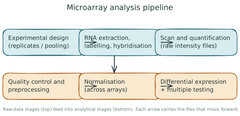
The microarray analysis workflow. Raw-data stages (top) feed into analytical stages (bottom).
The six stages shown are the steps this lecture covers in sequence.
Pre-processing
Preprocessing
Adjusting systematic effects due to technology variation, not biology variation.
Background Correction.
Normalization.
Summarization (some platforms).
Background correction
Background correction
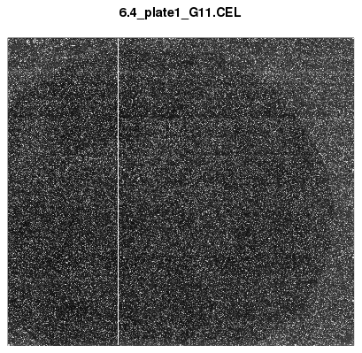
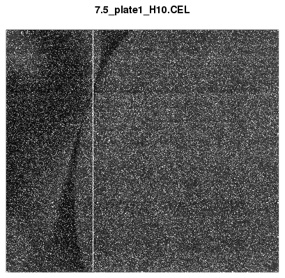
Subtraction of the background intensities from the foreground at each spot. Analysis per-sample.
Exploratory Analysis (1/5)
Exploratory Analysis (2/5)
Exploratory Analysis (3/5)
Exploratory Analysis (4/5)
Exploratory Analysis (5/5)
Normalization
Normalization
Remove systematic variation from the data, scaling data so that comparison can be made across samples.
It is a critical step.
Normalization Between Arrays, and Within Arrays.
Normalization within arrays
Post Normalization within arrays
Pre-processing
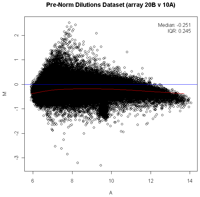
Red/green intensity ratio (M)
M = log_2(R/G)=log_2 R - log_2 G
Average intensity (A)
A= \frac{1}{2}log_2(RG)=\frac{log_2 R + log_2 G}{2}
MA Plots
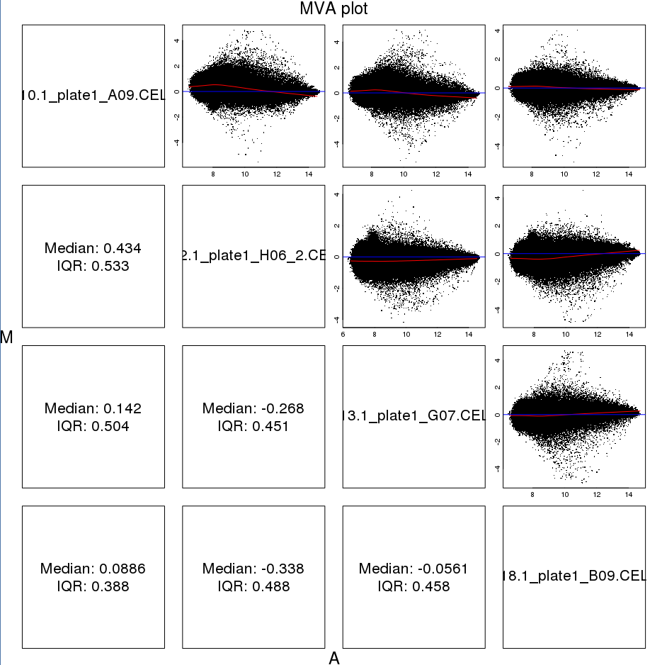
Prior to Normalization Between Arrays (1/2)
Pairwise scatter plots before between-array normalisation.
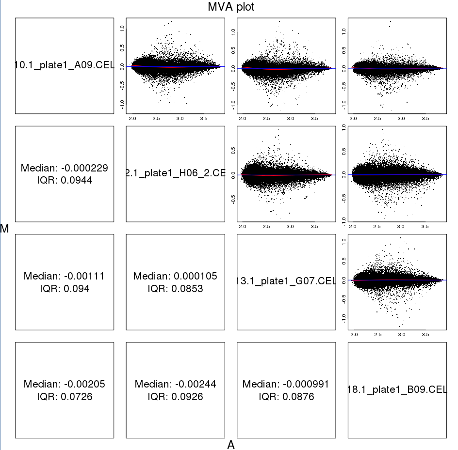
After Normalization Between Arrays
Pairwise scatter plots after between-array normalisation.
Microarray preprocessing methods
RMA
Background adjustment, quantile normalisation, and robust probe-set summarisation on the log scale.
GC-RMA
Extends background modelling to account for probe sequence composition and non-specific binding.
Li–Wong model
Model-based expression estimation accounts for probe-specific response. It is distinct from loess smoothing.
The appropriate method depends on array platform and experimental design.
Analysis of Differential Expression
Two approaches
Classical statistical tests.
Linear models.
Classical statistical tests
workflow
Generate Hypothesis.
Choose appropriate statistical test.
Compute p-value.
Correct for multiple testing.
Decide on confidence p-value threshold.
List selected.
Choosing a t-test
Comparison
Test
One group mean against a specified value
One-sample t-test
Matched or repeated measurements
Paired t-test on within-pair differences
Two independent group means
Welch two-sample t-test
The pooled-variance test additionally assumes equal population variances. Inspect the study design, sample size, and distribution of errors or differences.
One-sample t-test (1/2)
t-statistic:
t=\frac{\bar X - \mu}{ \sigma /_{\sqrt{n}} }
x <-rnorm(100, mean=2,sd=0.5)t.test(x)
    One Sample t-test

data:  x
t = 38.277, df = 99, p-value < 2.2e-16
alternative hypothesis: true mean is not equal to 0
95 percent confidence interval:
 1.936873 2.148657
sample estimates:
mean of x
 2.042765
One-sample t-test (2/2)
x <-rnorm(100, mean=0,sd=0.5)t.test(x)
    One Sample t-test

data:  x
t = 1.7802, df = 99, p-value = 0.07811
alternative hypothesis: true mean is not equal to 0
95 percent confidence interval:
 -0.01084199  0.20005835
sample estimates:
 mean of x
0.09460818
    Two Sample t-test

data:  x and y
t = -0.53311, df = 18, p-value = 0.3002
alternative hypothesis: true difference in means is less than 0
95 percent confidence interval:
     -Inf 2.027436
sample estimates:
mean of x mean of y
     11.4      12.3
Two-sample t-tests (3/3)
t.test(x,y,alt="less")
    Welch Two Sample t-test

data:  x and y
t = -0.53311, df = 16.245, p-value = 0.3006
alternative hypothesis: true difference in means is less than 0
95 percent confidence interval:
     -Inf 2.044664
sample estimates:
mean of x mean of y
     11.4      12.3
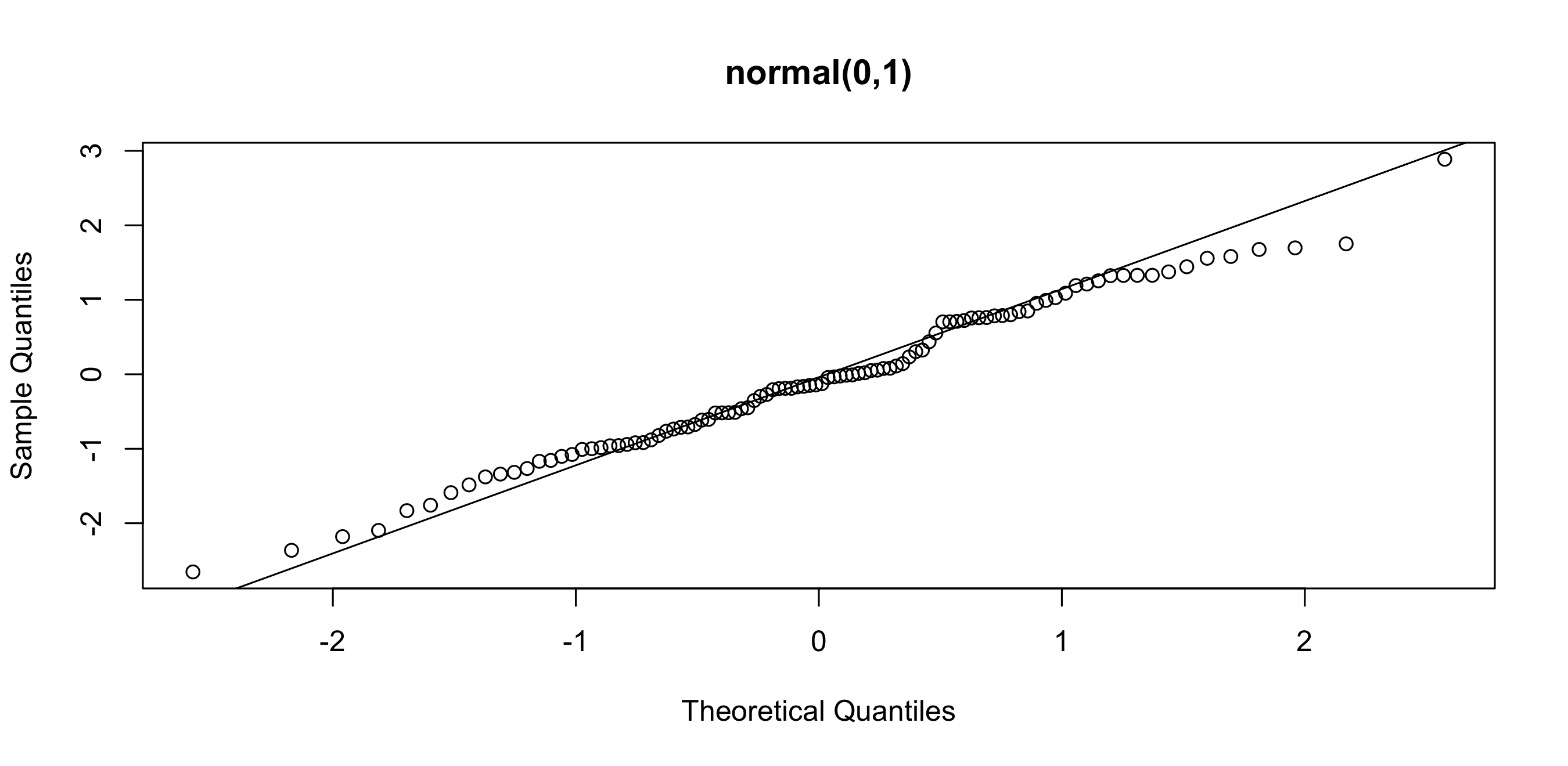
Non-Gaussian Data: Q–Q plots (1/2)
x =rnorm(100,0,1);qqnorm(x,main='normal(0,1)');qqline(x)
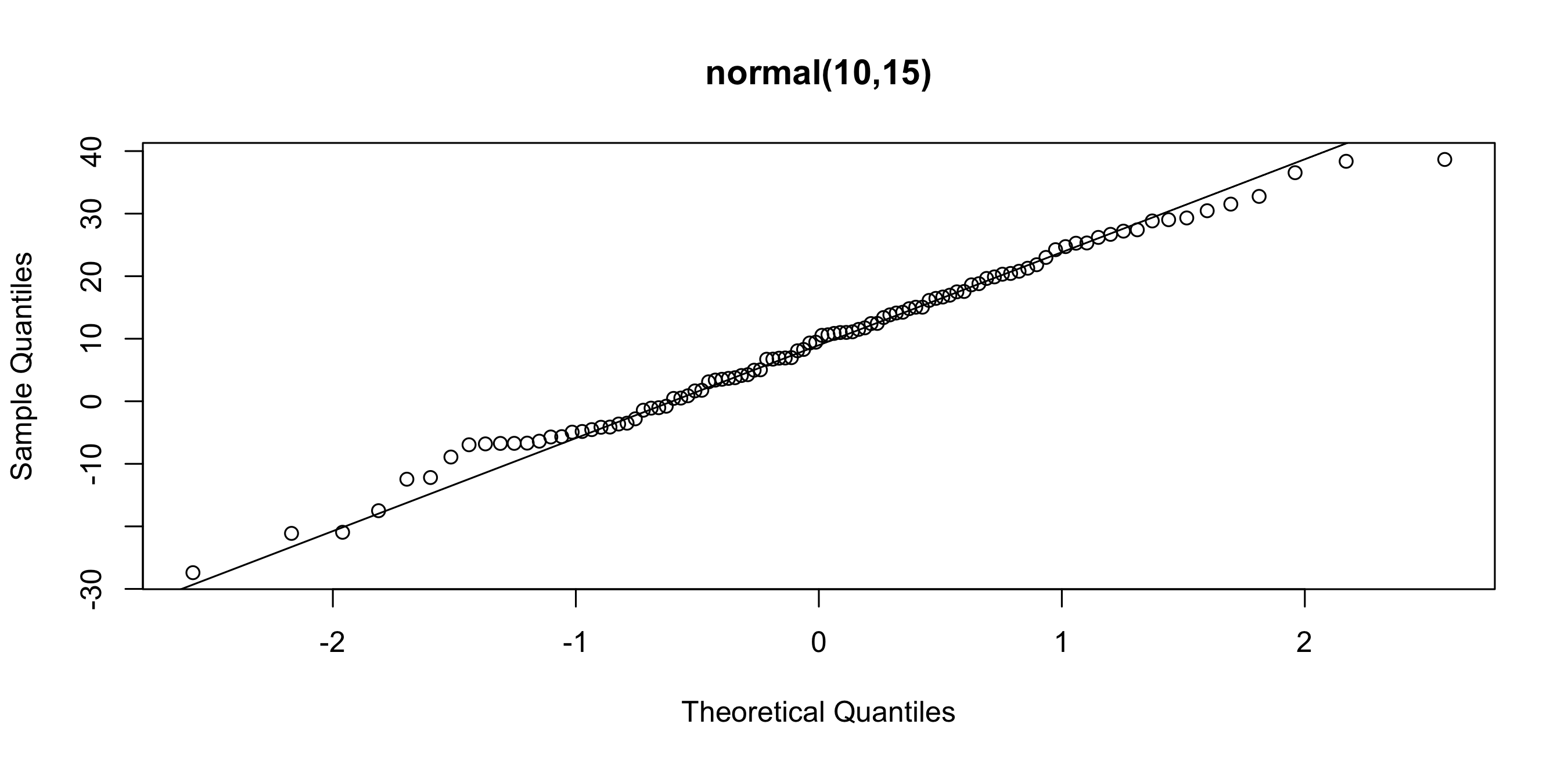
Non-Gaussian Data: Q–Q plots (2/2)
x =rnorm(100,10,15);qqnorm(x,main='normal(10,15)');qqline(x)
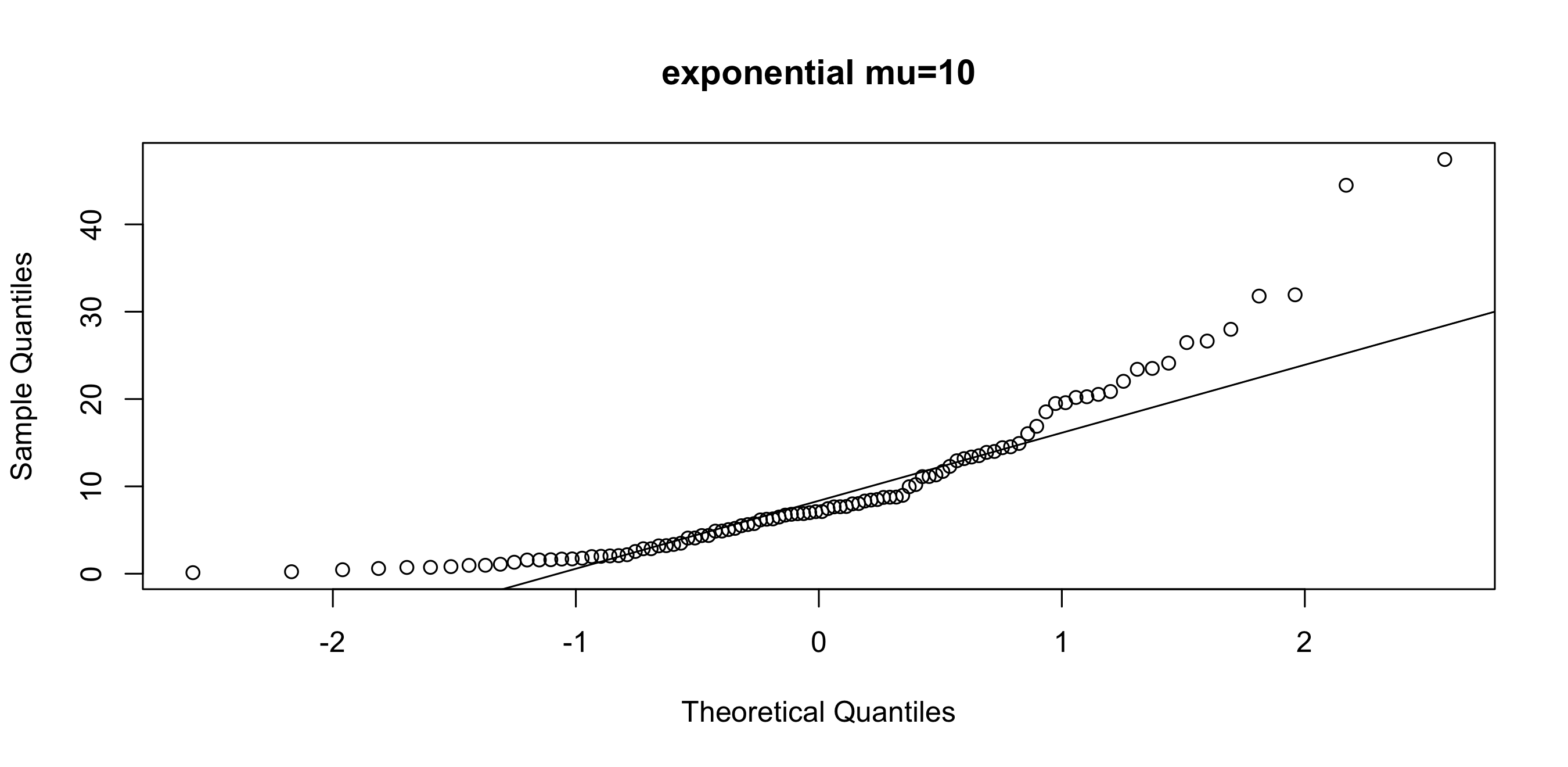
Non-Gaussian data: Q–Q plots (1/2)
x =rexp(100,1/10);qqnorm(x,main='exponential mu=10');qqline(x)
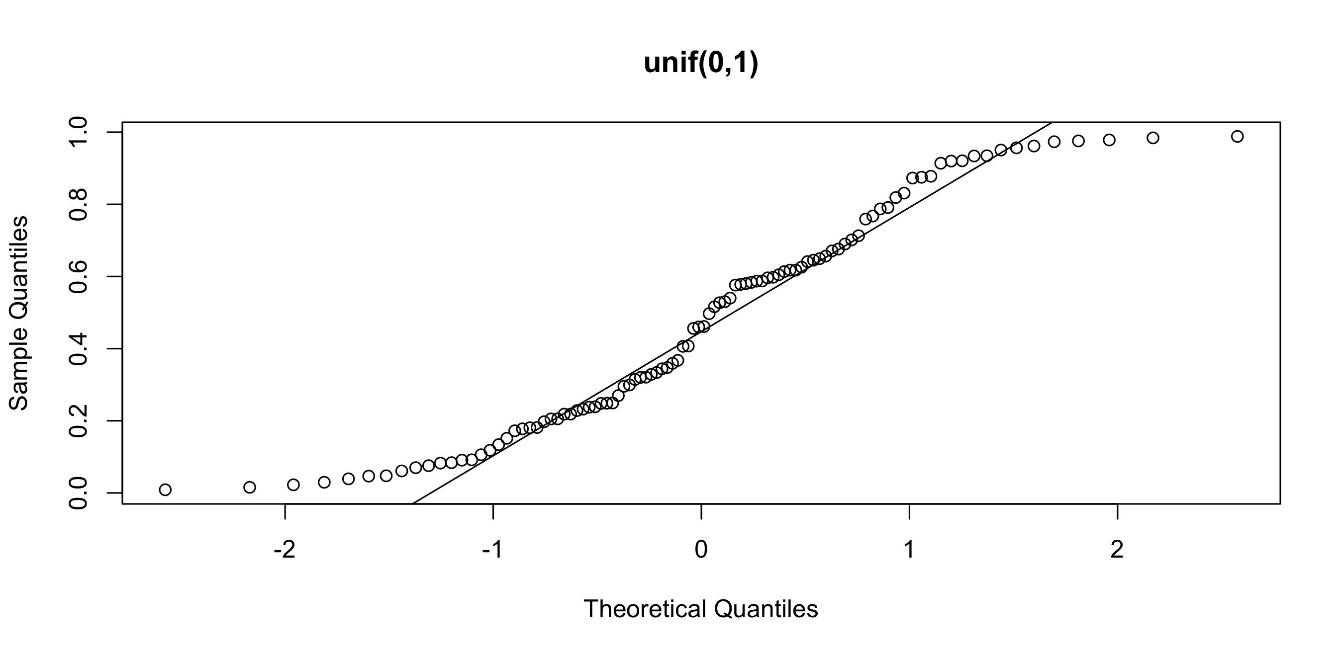
Non-Gaussian data: Q–Q plots (2/2)
x =runif(100,0,1);qqnorm(x,main='unif(0,1)');qqline(x)
Rank-based tests
Mann–Whitney / Wilcoxon rank-sum
Compares two independent samples. Its general null concerns distributions; a median-shift interpretation needs additional shape assumptions.
Wilcoxon signed-rank
Uses paired differences and assumes a symmetric distribution of those differences for its usual location interpretation.
These tests can be used with small samples, but discreteness, ties, and the available exact or approximate method affect inference.
Chi-squared goodness-of-fit test (1/2)
Allows a statistical test for categorical data
\chi^2-test:
\chi^2 = \sum^n_{i=1} \frac{(f_i-e_i)^2}{e_i}
Assumption (Cochran’s rule): every expected count is at least 1, and no more than 20% of the cells have expected counts below 5.
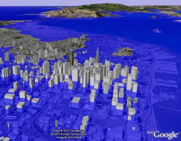
San Francisco under a flooded-sea scenario, visualised in Google Earth. As a metaphor: the “signal” (the city skyline) remains identifiable, but the surrounding “noise” (the raised sea) drowns everything at the same scale. When many hypotheses are tested, the noise floor rises with the number of tests — and a “significant” gene is a building that seems to rise above water, with no guarantee that it truly does.
Functional Enrichment
Enrichment techniques
Experimental data can be understood in the framework of the known biological context. Enrichment techniques relate this data to biological pathways.
Enrichment in gene expression
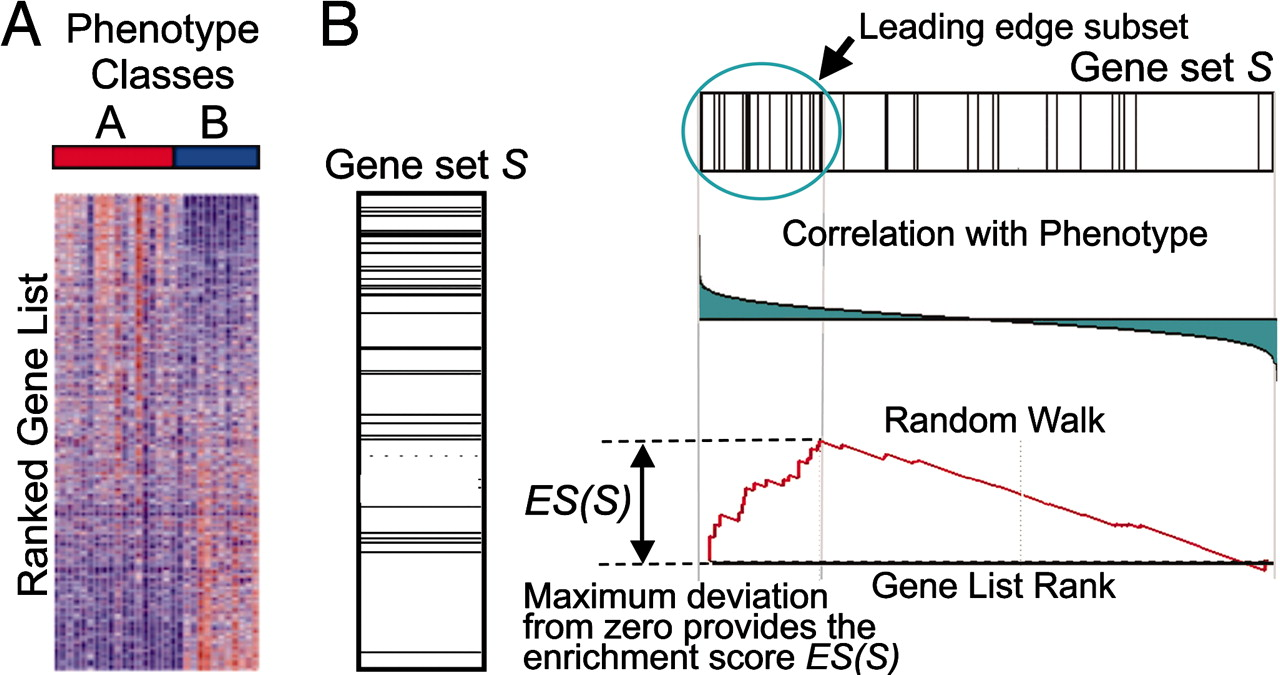
The challenge no longer lies in obtaining gene expression profiles, but rather in interpreting the results to gain insights into biological mechanisms.
(Subramanian et al PNAS 2005)
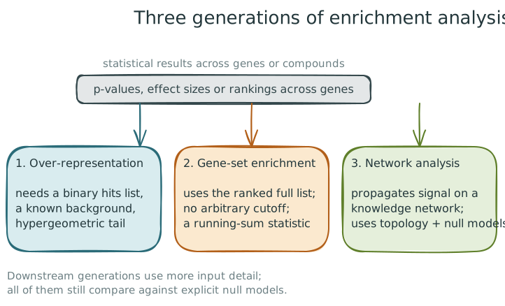
Three generations appear on later slides: over-representation (binary hits list, known background), gene-set enrichment (ranked full list, no cutoff), network analysis (signal propagated over a knowledge network).
Databases
Genes and gene products
Gene Ontology: contains three ontologies and a hierarchical structure reflecting the specificity of the entry (The Gene Ontology Consortium, NAR 2008).
Proteomics
UniProt: comprehensive database for protein sequence and annotation data (The UniProt Consortium, NAR 2018).
STRING: protein association database, including functional and physical associations; automatic and curated evidence (von Mering et al, NAR 2005).
Metabolomics
KEGG: comprehensive and curated pathway database (Kanehisa, NAR 2000).
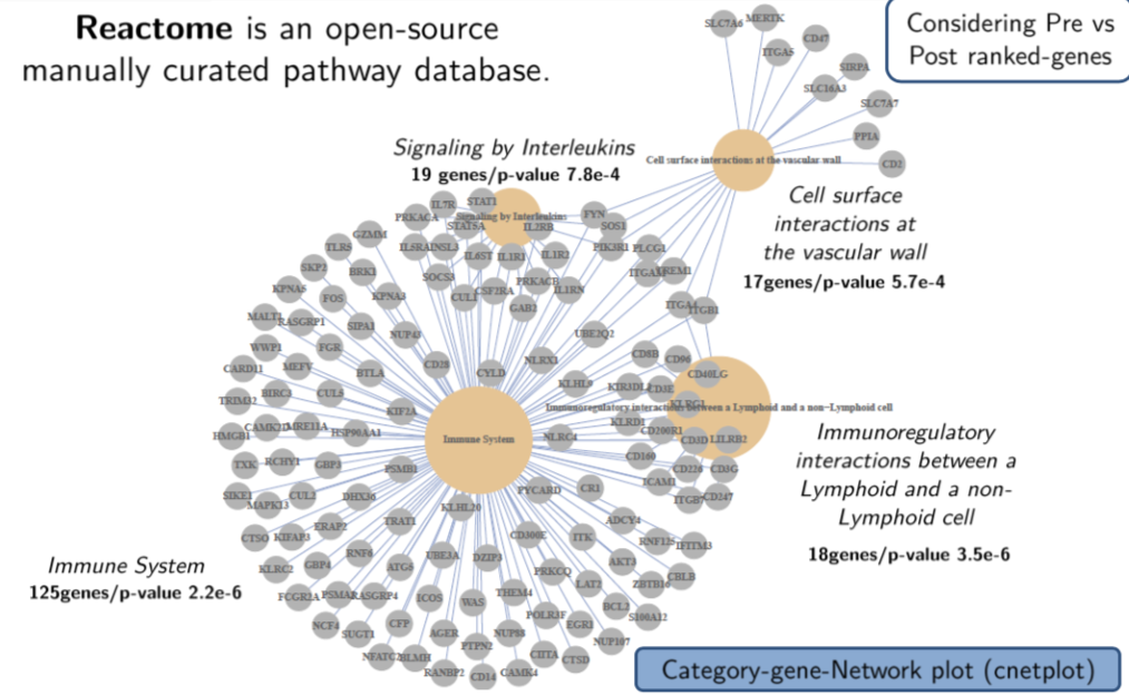
Reactome, BioCyc, WikiPathways, SMPDB
Gene Ontology
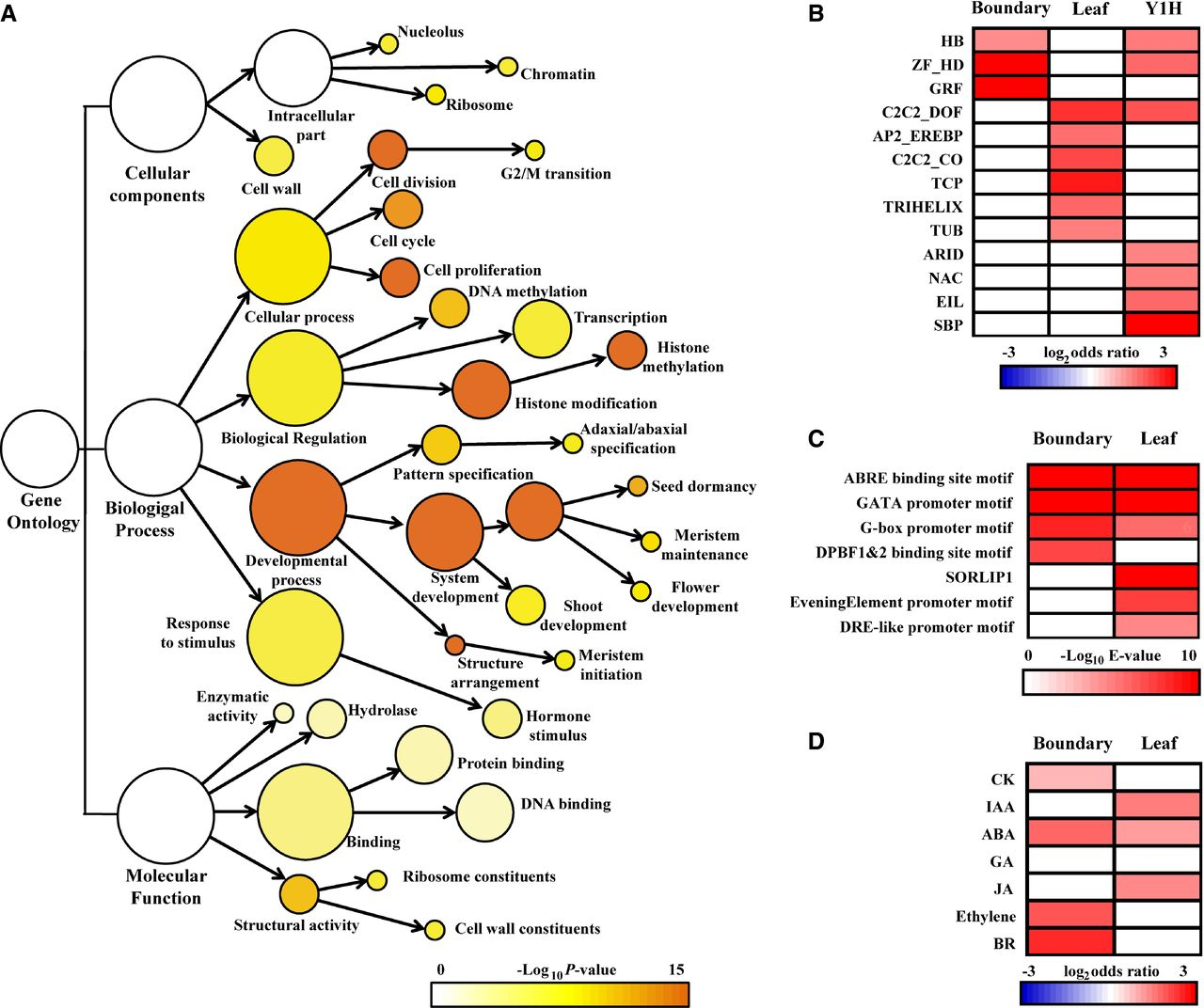
An example of GO overrepresentation analysis (ORA) (Tian 2014).
Over-representation analysis
Define a background of N genes that could have been selected. A pathway contains K of these genes; the selected list has n genes, with overlap k.
\log \frac{1}{p} incorporates a p-value from over-representation analysis in the original Pathway-Express formulation
PF(g) = \Delta E (g) + \sum\limits_{u \in US_g} \beta_{ug} \cdot \frac{PF(u)}{N_{ds}(u)} considers the topology of the genes within the pathway, and is similar to PageRank scores.