Pattern recognition
Bioinformatics · Universitat Politècnica de Catalunya
Data
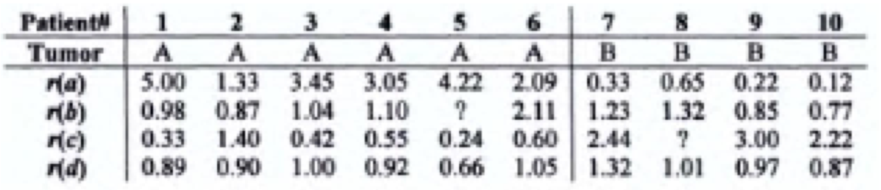
Note the missing values…
Data
Data
Data
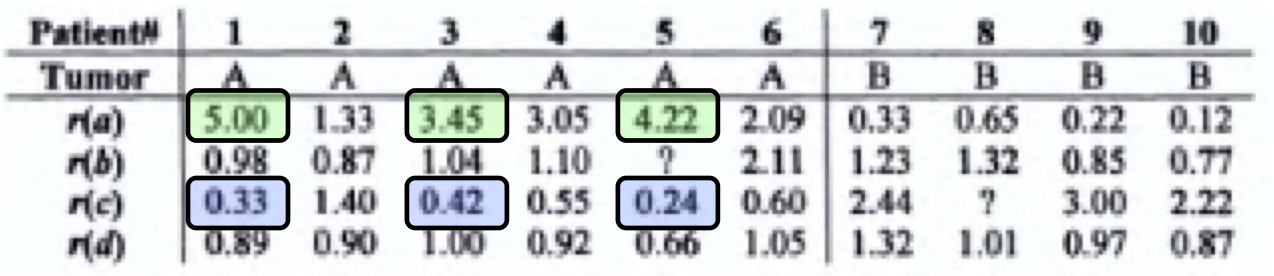
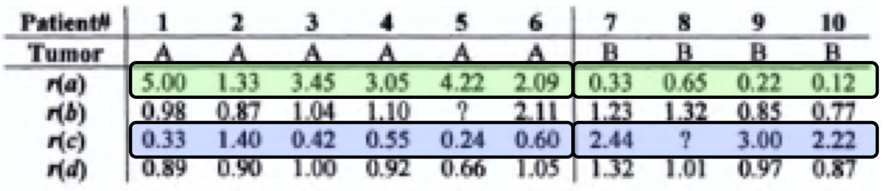
Note that r(a) and r(c) are both negatively co-regulated…
Data and Goals
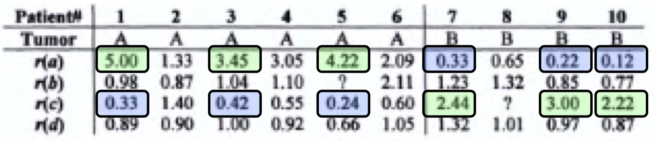
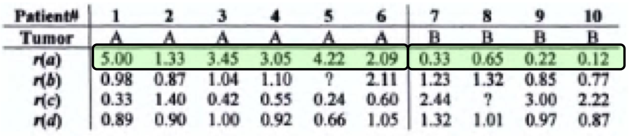
Could we guess the most involved genes in the Cancer process differentiation?
Given a readout with the expression values for a,b,c,d genes, can we predict whether a new patient has tumor A or B?
Pattern Recognition Scheme in classification (1/3)

Pattern Recognition Scheme in classification (2/3)
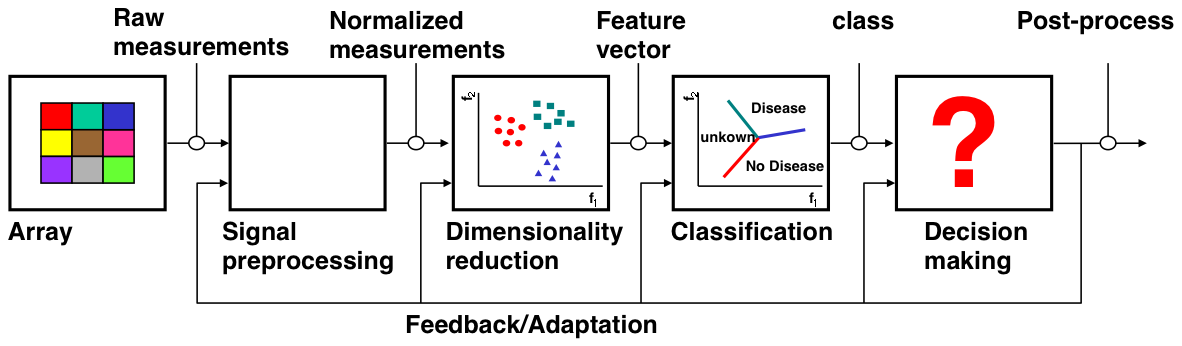
Pattern Recognition Scheme in classification (3/3)

The curse of Dimensionality (1/2)
Term coined by Bellman (1961)
Describes a problem related with the relationship of multivariate data and number of samples
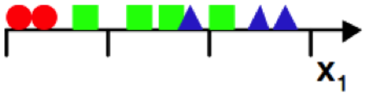
Consider a 3-class pattern recognition
One feature or variable.
![The curse of Dimensionality]()
The curse of Dimensionality (2/2)
The Easiest classifier: three bins / three samples per bin, then, vote
![The curse of Dimensionality]()
Can we improve the classification performance adding a second feature?

Adapted from Gutierrez-Osuna
Curse of Dimensionality
We shall maintain the density of examples we used on the 1D case?
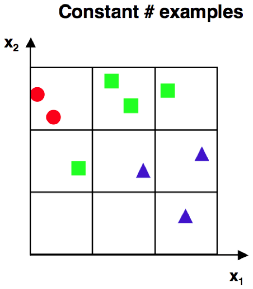
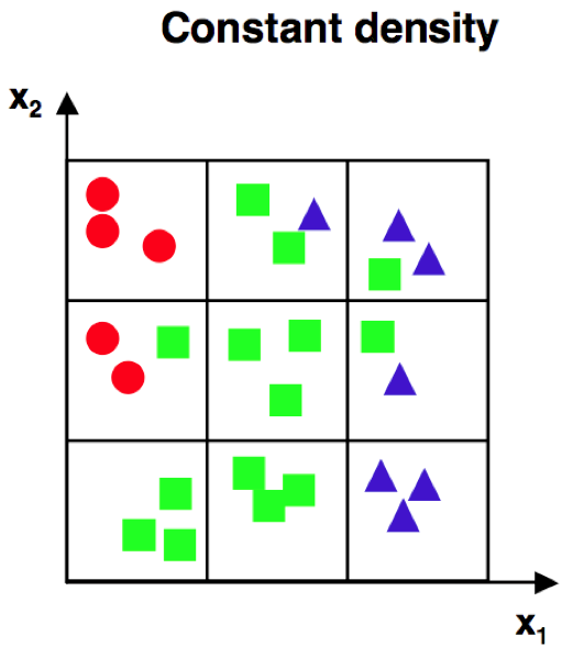
Bins are now 9 -> we will need 27 samples to maintain density.
on 3d, 27bins, 81 samples…
Adapted from Gutierrez-Osuna
The Curse of Dimensionality
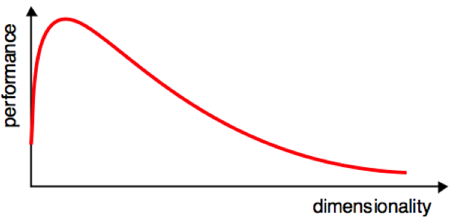
Houston! We…
How could we avoid the curse of dimensionality?
Using prior knowledge.
Smoothing the target function.
Reducing the dimensionality.
Feature Selection vs Feature Extraction
Feature Selection
From a set of input N variables, select those which contain the most informative to the problem
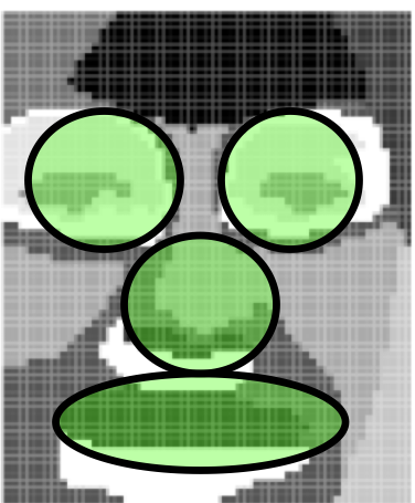
Feature Extraction
From a set of input N variables, could we define a set of functions or transformations that contains relevant information for our problem?
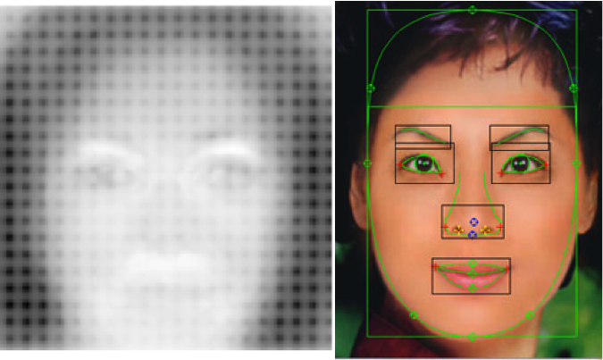
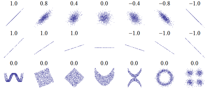
Pearson
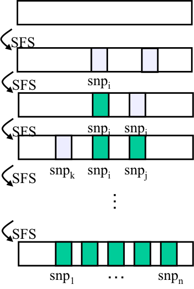
Sequential Selection Algorithms (1/3)
Sequential Selection Algorithms (2/3)
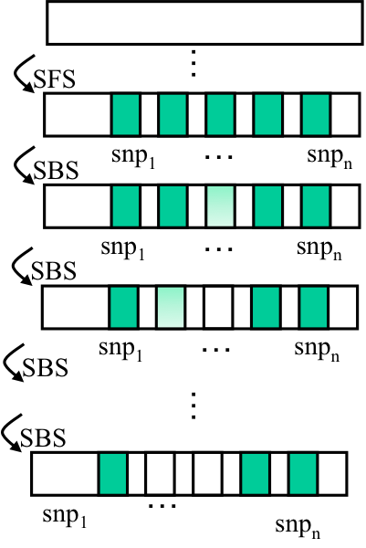
Sequential Selection Algorithms (3/3)
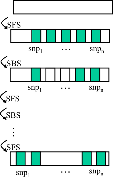
Can redundant variables help each other?
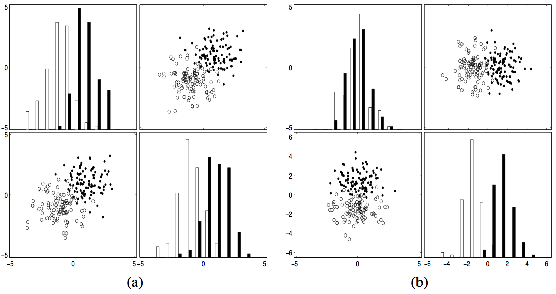
(a): The presumably redundant variables, (b) set after a 45 degree rotation
from Guyon 2003
Intra-Class covariance
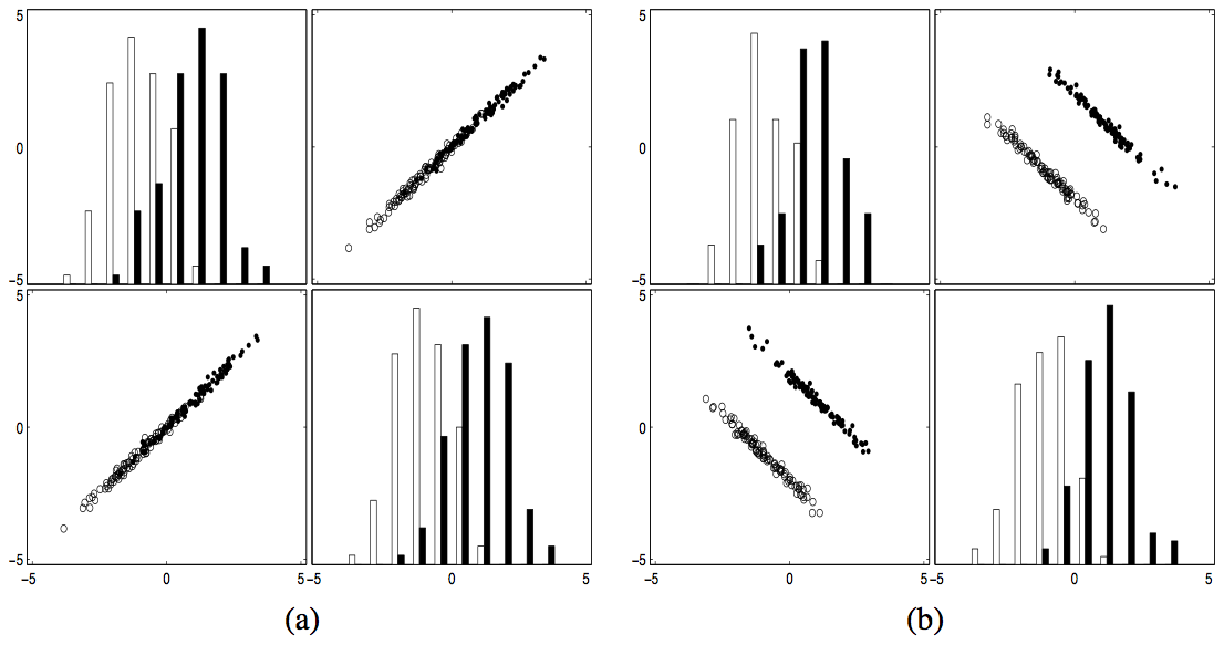
(a) The class conditional distributions have a high covariance aligned with two class centers. (b) The class conditional distributions have a high covariance in the direction perpendicular to the line of the two class centers.
from Guyon 2003
Is covariance useful?
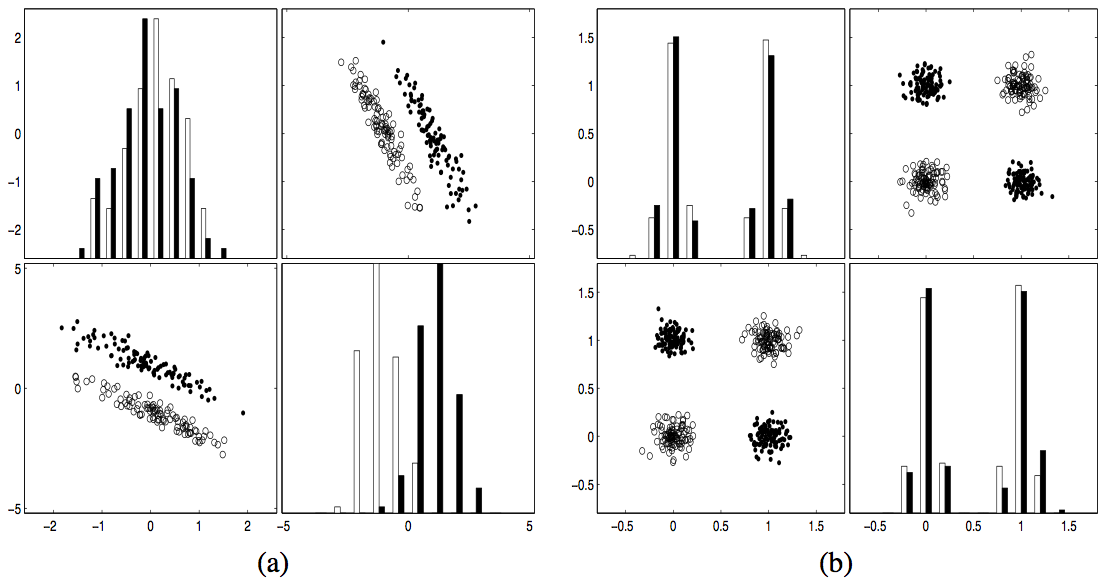
from Guyon 2003
Feature extraction: subspace methods
Project observations into a lower-dimensional representation that retains information relevant to the task.
Examples include:
- Principal component analysis (PCA)
- Linear discriminant analysis (LDA)
- Independent component analysis (ICA)
Each method uses a different criterion; dimension reduction does not automatically preserve predictive information.
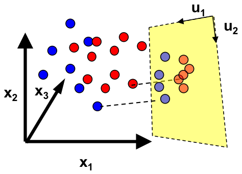
Principal Component Analysis
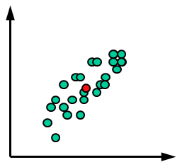
Principal Component Analysis
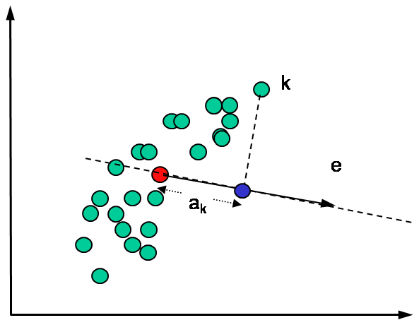
PCA
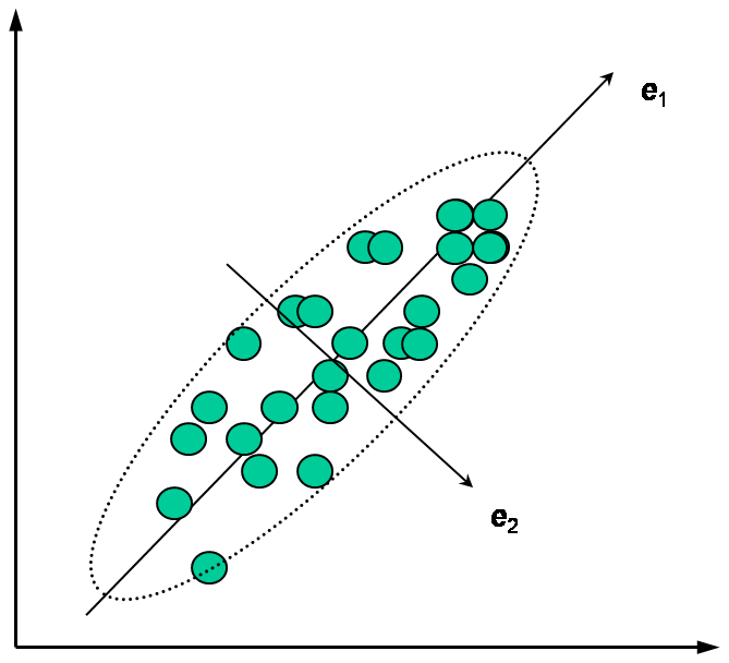
PCA (1/4)
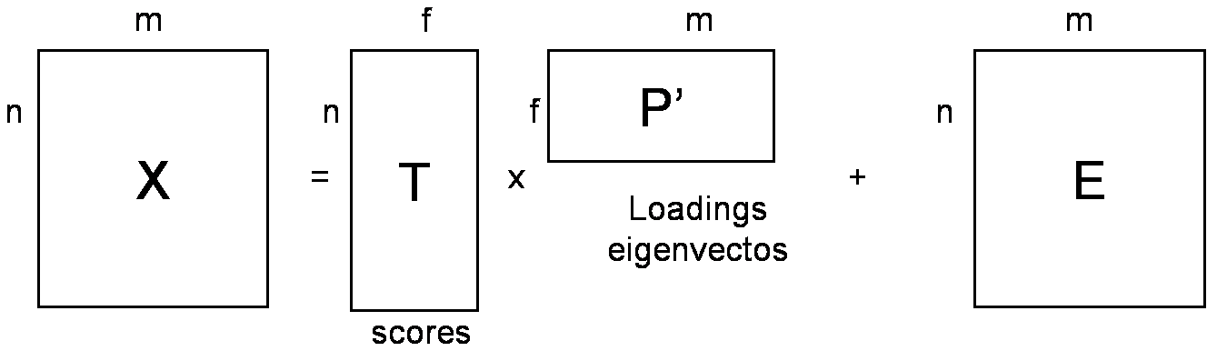
PCA (2/4)
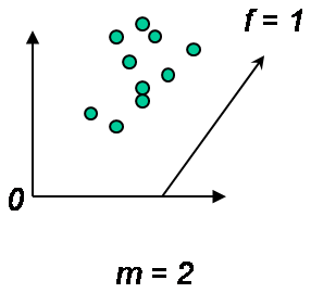
PCA (3/4)
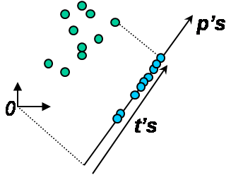
PCA (4/4)
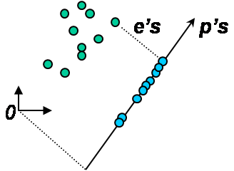
PCA
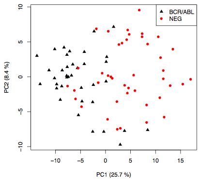
Linear Discriminant Analysis
LDA minimizes the within scatter matrix while maximizes the between scatter matrix.
It can be extended to Multiple classes (Multiple Discriminant Analysis)
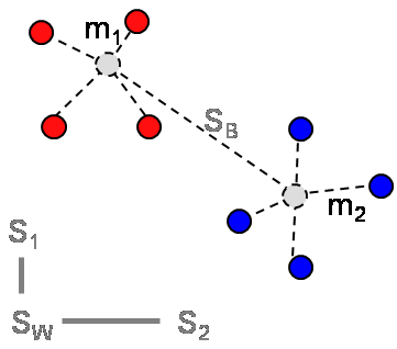
LDA vs PCA (1/4)
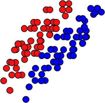
LDA vs PCA (2/4)
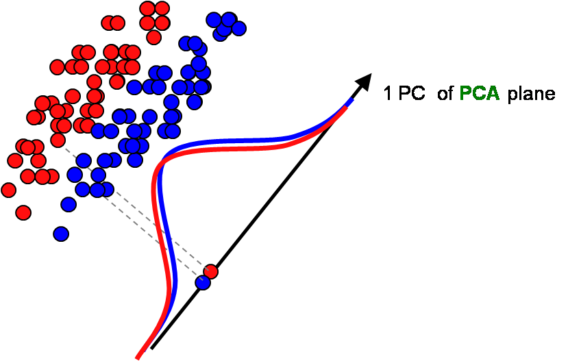
LDA vs PCA (3/4)
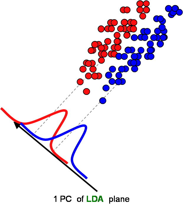
LDA vs PCA (4/4)
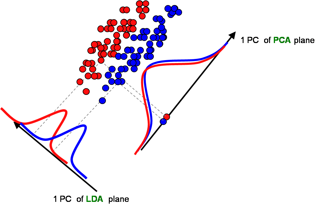
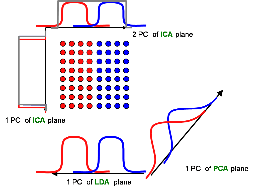
LDA vs PCA vs ICA (1/4)
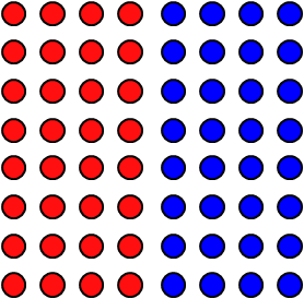
LDA vs PCA vs ICA (2/4)
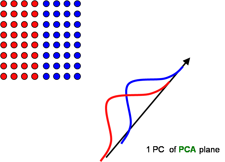
LDA vs PCA vs ICA (3/4)
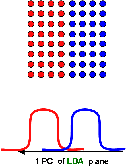
LDA vs PCA vs ICA (4/4)
Nonlinear class boundaries
There are non-linear problems:
Can be linearized?
Can we change the features measured?
Representation change?
If “no”, then there are non-linear alternatives.
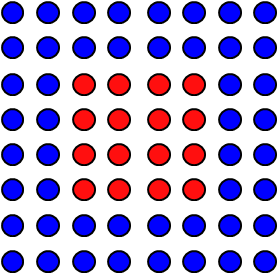
k-NN (1/4)
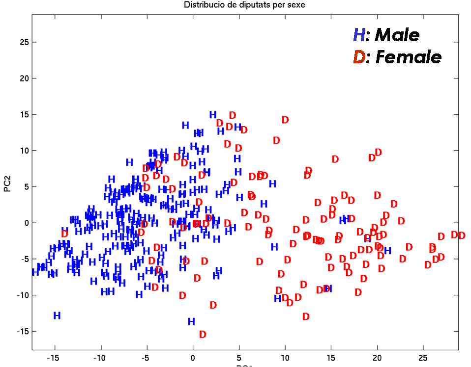
k-NN (2/4)
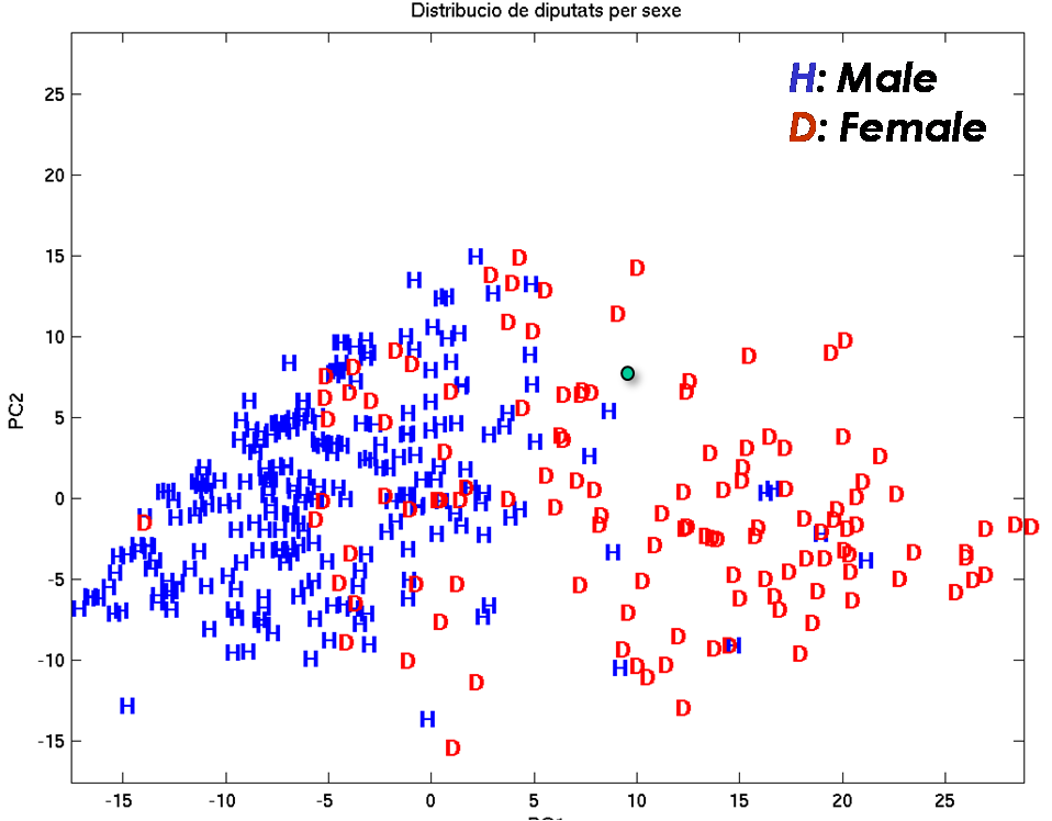
k-NN (3/4)
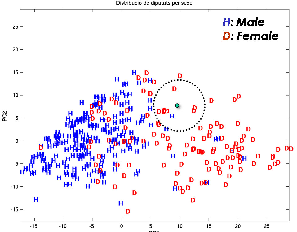
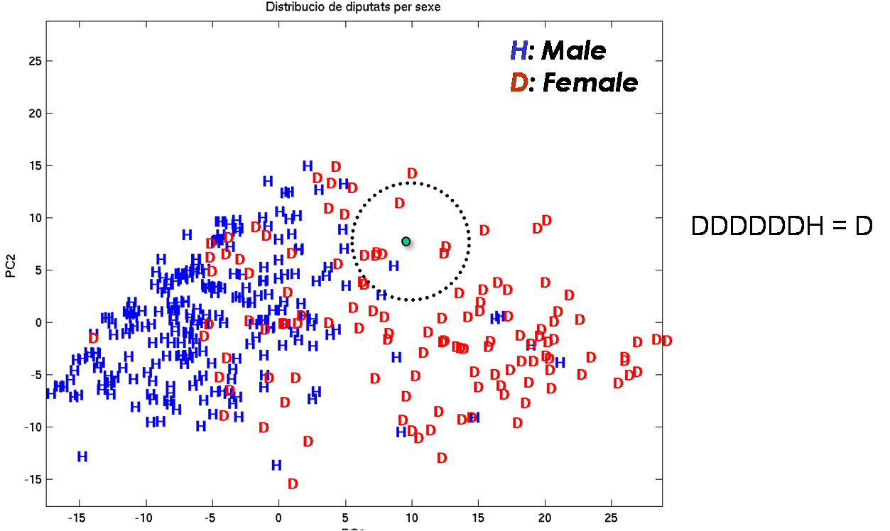
k-NN (4/4)
Voronoi Tessellation
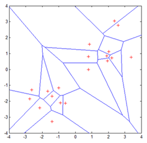
Voronoi Tessellation
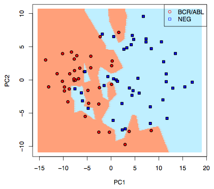
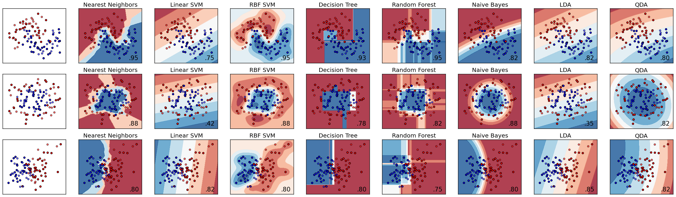
Classification algorithms in sklearn
Clustering (1/5)
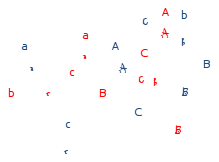
Clustering (2/5)
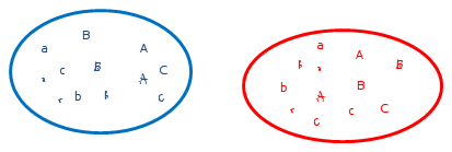
Clustering (3/5)
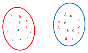
Clustering (4/5)
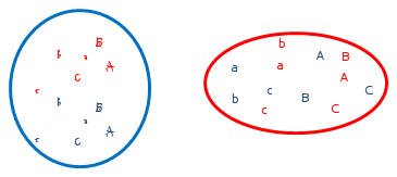
Clustering (5/5)
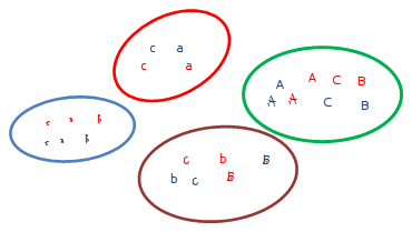
Clustering

kmeans (1/10)
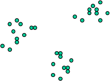
kmeans (2/10)
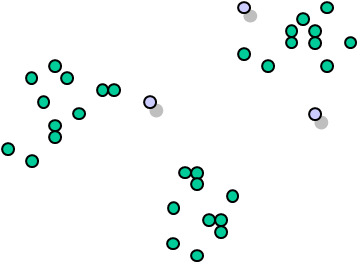
kmeans (3/10)
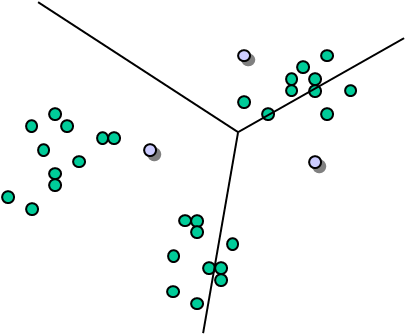
kmeans (4/10)
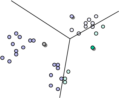
kmeans (5/10)
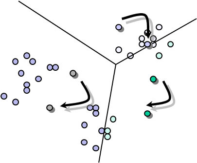
kmeans (6/10)
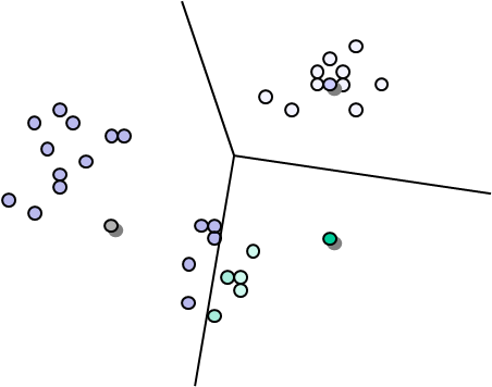
kmeans (7/10)
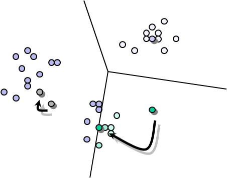
kmeans (8/10)
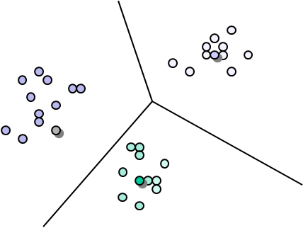
kmeans (9/10)
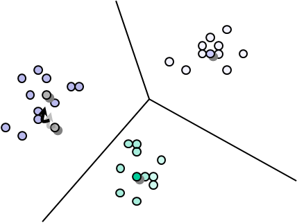
kmeans (10/10)
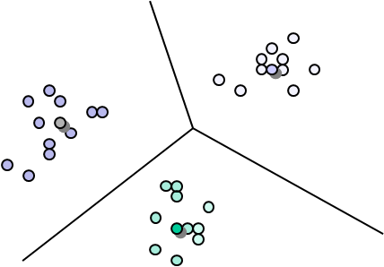
kmeans
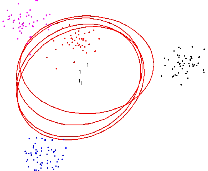
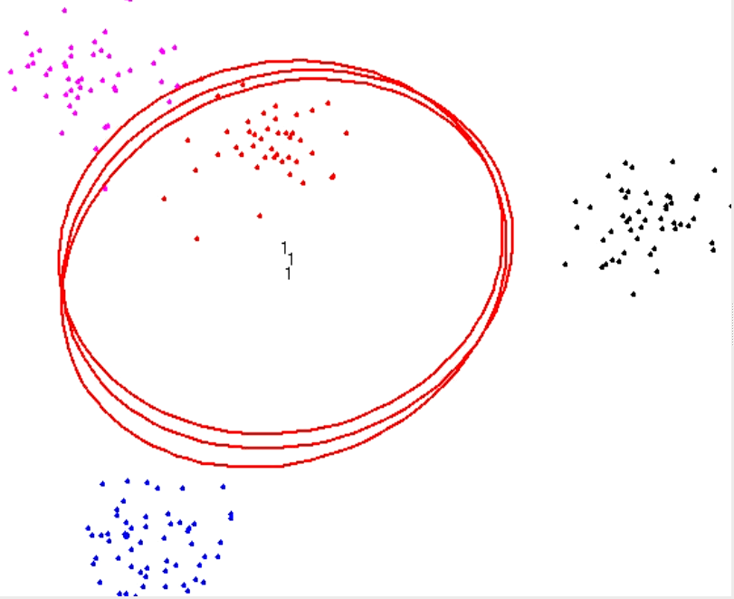
Number of Clusters
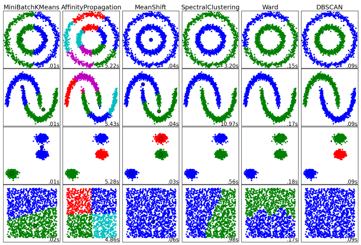
Clustering algorithms in sklearn
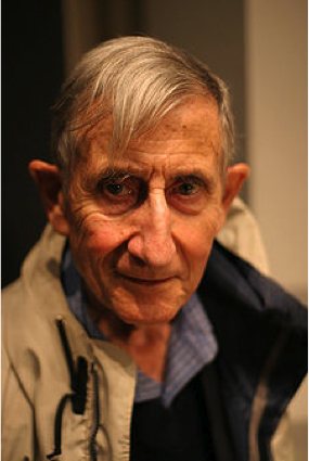
Fermi
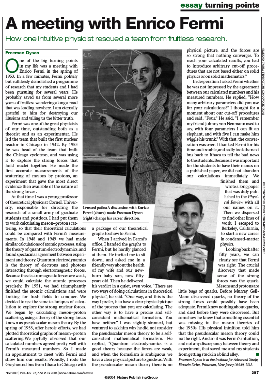
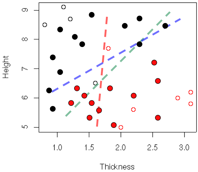
over-fitting (2/3)
+ 
over-fitting (3/3)
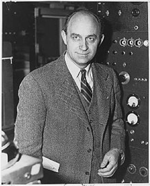
From Dyson, F. A meeting with Enrico Fermi; how one intuitive physicist rescued a team from fruitless research. Nature 2004.
Over-Fitting
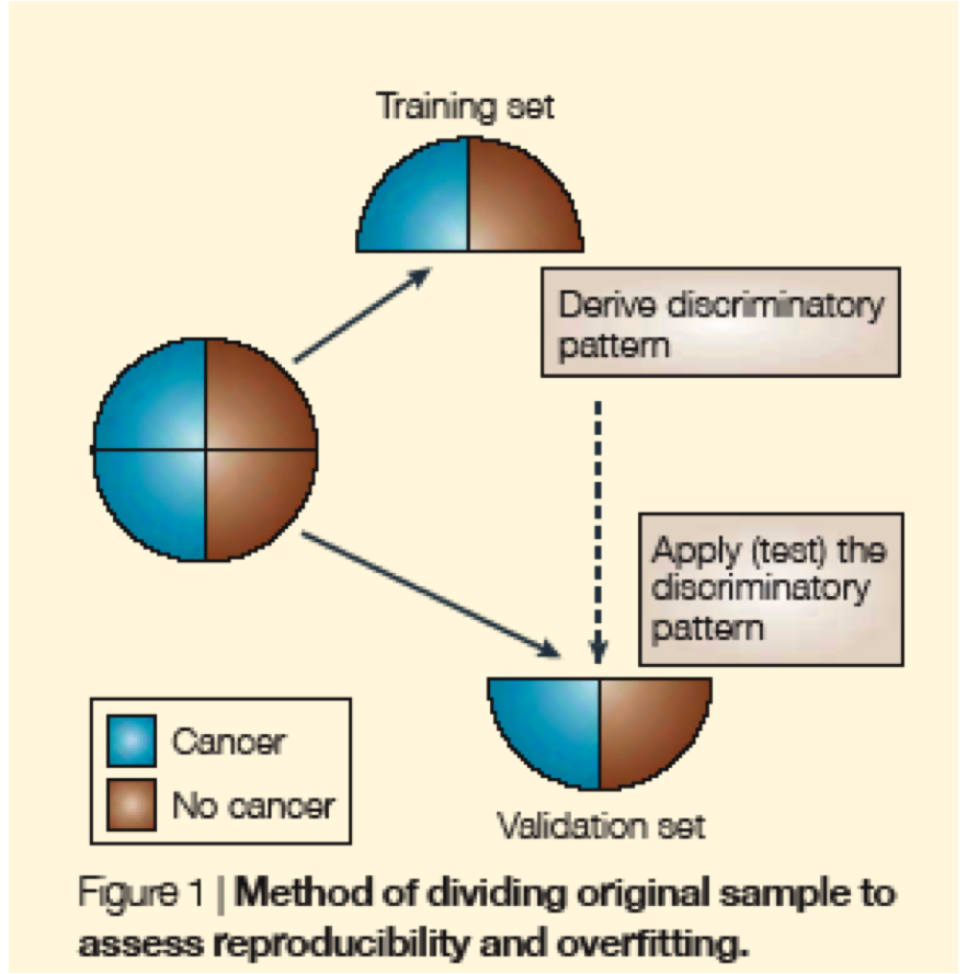
Validation Schemes
Ransohoff. Nat Rev Cancer 2004
Validation without leakage
Fit preprocessing, feature selection, and tuning using only the training partition. For tuned models, use nested cross-validation or an untouched test set. Keep samples from the same person together when splitting.