             Species Endemics  Area Elevation Nearest Scruz Adjacent
Baltra            58       23 25.09       346     0.6   0.6     1.84
Bartolome         31       21  1.24       109     0.6  26.3   572.33
Caldwell           3        3  0.21       114     2.8  58.7     0.78
Champion          25        9  0.10        46     1.9  47.4     0.18
Coamano            2        1  0.05        77     1.9   1.9   903.82
Daphne.Major 18 11 0.34 119 8.0 8.0 1.84Linear models in R
Bioinformatics · Universitat Politècnica de Catalunya
Alexandre Perera-Lluna
What makes a model linear?
A linear model is linear in its unknown coefficients:
Y=\beta_0+\beta_1X_1+\beta_2\log(X_2)+\beta_3X_1X_3+\varepsilon.
Predictor transformations and interactions are allowed.
By contrast, Y=\beta_0+\beta_1X_1^{\beta_2}+\varepsilon is nonlinear in the unknown exponent \beta_2.
Linear models in matrix form
y=X\beta+\varepsilon,\qquad \hat y=X\hat\beta.
- y: n\times1 response vector.
- X: n\times q design matrix, including the intercept when present.
- \beta: q\times1 coefficient vector.
- Least squares minimises \lVert y-X\beta\rVert^2.
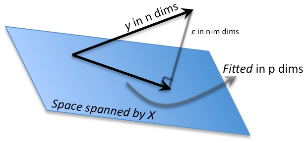
For a full-rank design, fitted residuals are orthogonal to the columns of X and have n-q residual degrees of freedom. The random error vector itself is not constrained to that residual subspace.
Geometrical representation
Formula notation in R
It is possible to use a formula notation in R, when these are named (
names()).In previous example:
Sepal.Length ~ SpeciesFormulas in R
variable \sim group
variables per group
This notation is homogeneous along most of R code
Formula Notation in R, II
Formulas
response \sim model
See
help(formula)log(Sepal.Length) ~ SpeciesArithmetic functions are allowed:
I(Sepal.Length + Petal.Length) ~ SpeciesHeavily used in linear regression, but also in visualization functions
Galápagos plant species data
Galápagos Islands : 30 islands, 7 variables
Species: The number of plant species found on the island
Area: The area of the island (km^2)
Nearest: The distance from the nearest island (km)
Elevation: The highest elevation of the island (m)
Endemics: The number of endemic species
Scruz: The distance from Santa Cruz island (km)
Adjacent: the area of the adjacent island (square km)
lm()
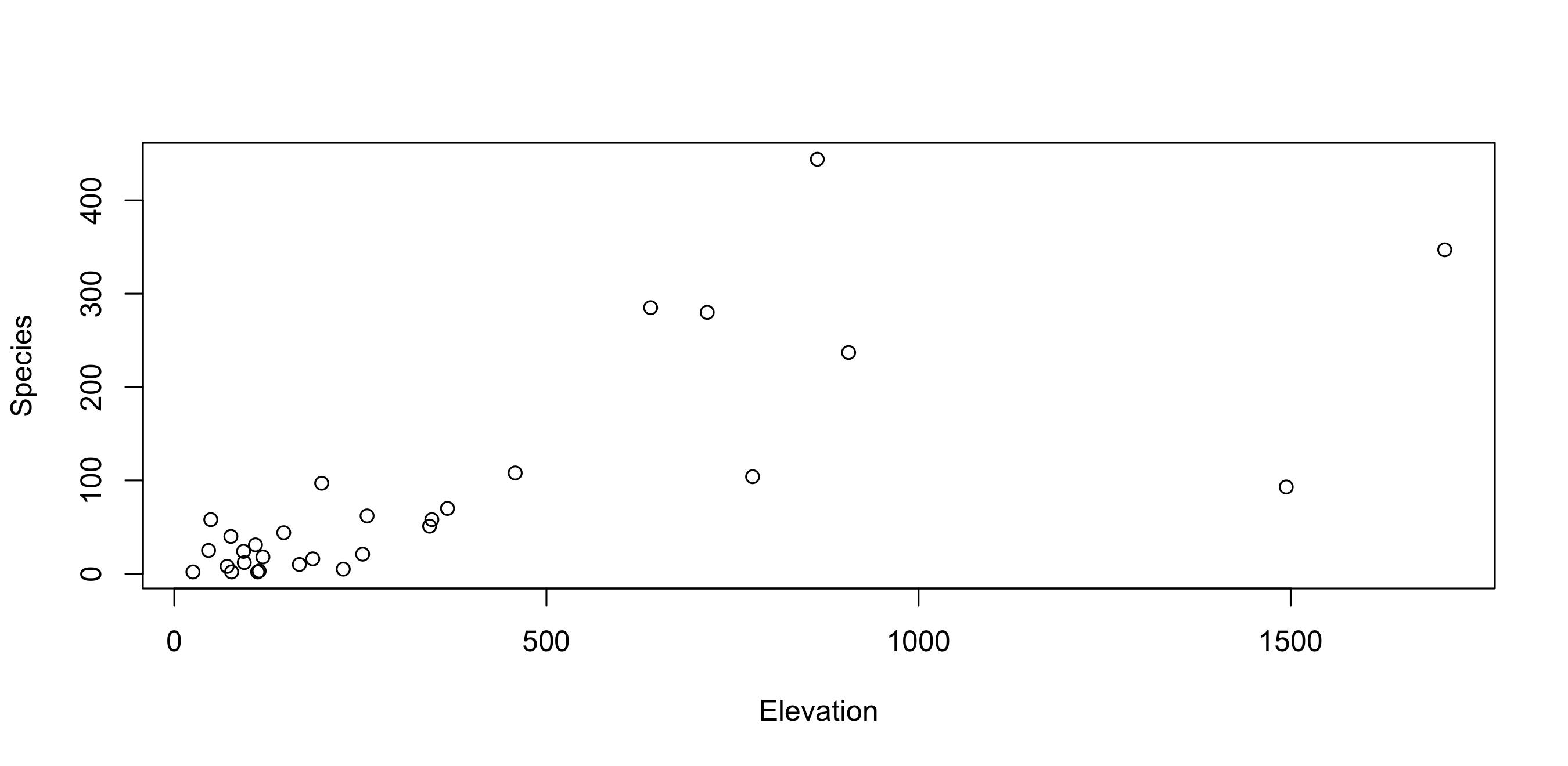
lm(): model construction (1/2)
lm(): model construction (2/2)
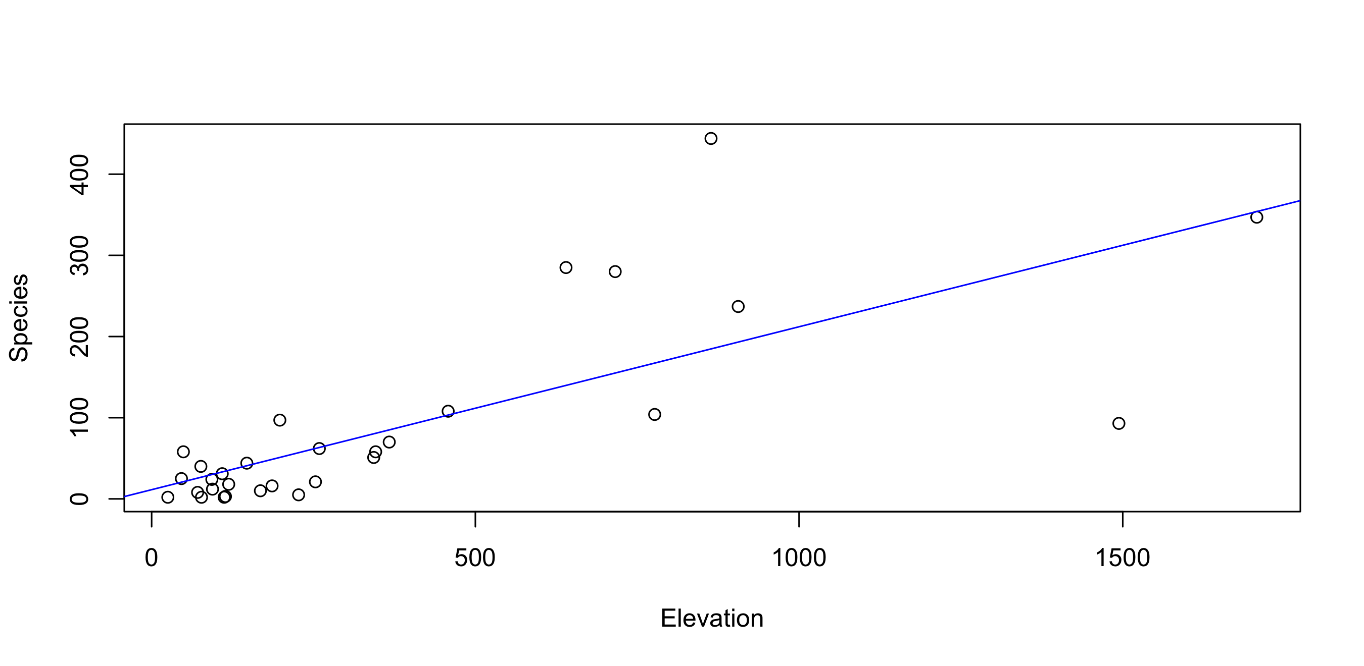
lm(): model information
Call:
lm(formula = Species ~ Elevation, data = gala)

Residuals:
     Min       1Q   Median       3Q      Max
-218.319  -30.721  -14.690    4.634  259.180

Coefficients:
            Estimate Std. Error t value Pr(>|t|)
(Intercept) 11.33511   19.20529   0.590     0.56
Elevation    0.20079    0.03465   5.795 3.18e-06 ***
---
Signif. codes:  0 '***' 0.001 '**' 0.01 '*' 0.05 '.' 0.1 ' ' 1

Residual standard error: 78.66 on 28 degrees of freedom
Multiple R-squared:  0.5454,    Adjusted R-squared:  0.5291
F-statistic: 33.59 on 1 and 28 DF, p-value: 3.177e-06lm(): plot(lm)
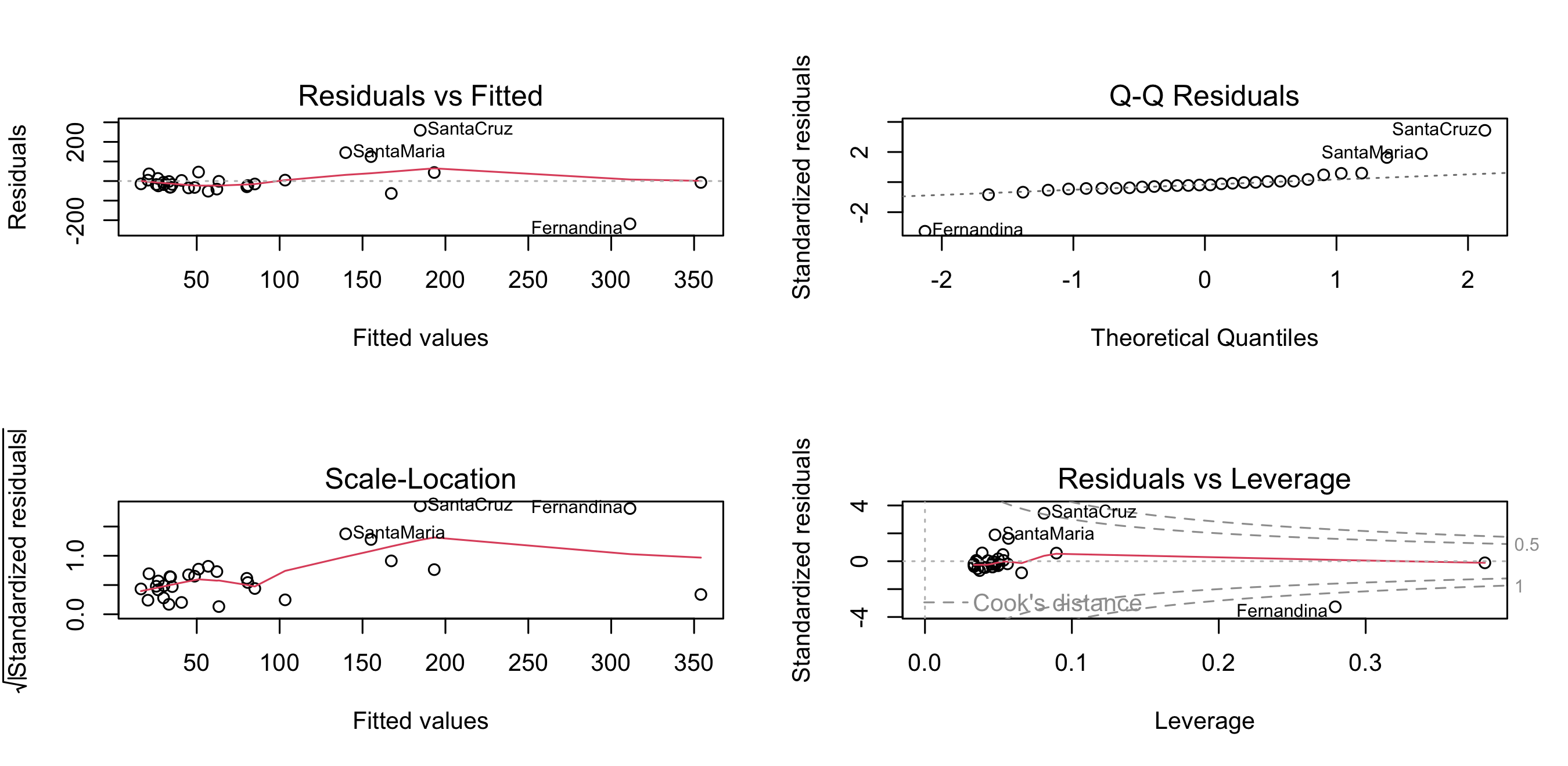
lm(): Residuals
      Baltra    Bartolome     Caldwell     Champion      Coamano Daphne.Major
  -22.809212    -2.221462   -31.225423     4.428446   -24.796112   -17.229384
Daphne.Minor       Darwin         Eden      Enderby     Espanola   Fernandina
   -6.008787   -35.068202   -17.591359   -31.823839    45.908033  -218.318650
    Gardner1     Gardner2     Genovesa      Isabela     Marchena       Onslow
   36.826069   -51.914941    13.404680    -7.087387   -29.206835   -14.354918
       Pinta       Pinzon   Las.Plazas       Rabida SanCristobal  SanSalvador
  -63.350647     4.702062   -18.209579   -15.025848   124.897677    43.747160
   SantaCruz      SantaFe   SantaMaria      Seymour      Tortuga         Wolf
259.180432 -1.340291 145.157883 3.148434 -32.682461 -41.135538 Durbin-Watson (1/2)
Evaluates Durbin-Watson for error auto-correlation
durbin.watson(car) Durbin-Watson Test for Autocorrelated Errors dwtest(lmtest) Durbin-Watson Test
Durbin-Watson (2/2)
lm(): Predictions
    Genovesa      Isabela     Marchena       Onslow        Pinta       Pinzon
    26.59532    354.08739     80.20684     16.35492    167.35065    103.29794
  Las.Plazas       Rabida SanCristobal  SanSalvador    SantaCruz      SantaFe
    30.20958     85.02585    155.10232    193.25284    184.81957     63.34029
  SantaMaria      Seymour      Tortuga         Wolf
139.84212 40.85157 48.68246 62.13554 lm(): Predictions, IC
                   fit         lwr       upr
Genovesa      26.59532  -3.2897506  56.48039
Isabela      354.08739 271.4761884 436.69858
Marchena      80.20684  55.7314194 104.68225
Onslow        16.35492 -15.3566679  48.06650
Pinta        167.35065 133.0307302 201.67056
Pinzon       103.29794  78.2982338 128.29764
Las.Plazas    30.20958   0.9226656  59.49649
Rabida        85.02585  60.5948667 109.45683
SanCristobal 155.10232 123.2045765 187.00007
SanSalvador  193.25284 153.2255598 233.28012
SantaCruz    184.81957 146.7231442 222.91599
SantaFe       63.34029  38.0783575  88.60222
SantaMaria   139.84212 110.6221988 169.06203
Seymour       40.85157  13.1644062  68.53873
Tortuga       48.68246  21.9996242  75.36530
Wolf 62.13554 36.7813407 87.48974lm(): Model construction
Call:
lm(formula = Species ~ Elevation + Endemics, data = gala)

Residuals:
   Min     1Q Median     3Q    Max
-74.85 -12.49   2.59  12.66  70.25

Coefficients:
             Estimate Std. Error t value Pr(>|t|)
(Intercept) -19.92862    7.14320  -2.790  0.00955 **
Elevation    -0.02294    0.02009  -1.142  0.26366
Endemics      4.35265    0.30997  14.042 6.29e-14 ***
---
Signif. codes:  0 '***' 0.001 '**' 0.01 '*' 0.05 '.' 0.1 ' ' 1

Residual standard error: 27.8 on 27 degrees of freedom
Multiple R-squared:  0.9452,    Adjusted R-squared:  0.9412
F-statistic: 233 on 2 and 27 DF, p-value: < 2.2e-16lm(): Model construction
Call:
lm(formula = Species ~ ., data = gala)

Residuals:
    Min      1Q  Median      3Q     Max
-68.219 -10.225   1.830   9.557  71.090

Coefficients:
              Estimate Std. Error t value Pr(>|t|)
(Intercept) -15.337942   9.423550  -1.628    0.117
Endemics      4.393654   0.481203   9.131 4.13e-09 ***
Area          0.013258   0.011403   1.163    0.257
Elevation    -0.047537   0.047596  -0.999    0.328
Nearest      -0.101460   0.500871  -0.203    0.841
Scruz         0.008256   0.105884   0.078    0.939
Adjacent      0.001811   0.011879   0.152    0.880
---
Signif. codes:  0 '***' 0.001 '**' 0.01 '*' 0.05 '.' 0.1 ' ' 1

Residual standard error: 28.96 on 23 degrees of freedom
Multiple R-squared:  0.9494,    Adjusted R-squared:  0.9362
F-statistic: 71.88 on 6 and 23 DF, p-value: 9.674e-14Principal Component Regression
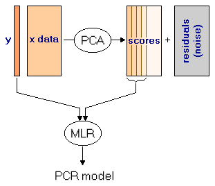
From H. Lohninger http://www.statistics4u.com
Principal Component Regression
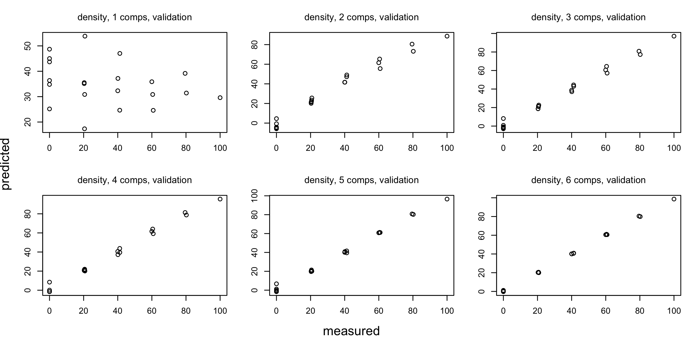
- Principal Component Regression:
pcr()enlibrary(pls)
Partial Least Squares
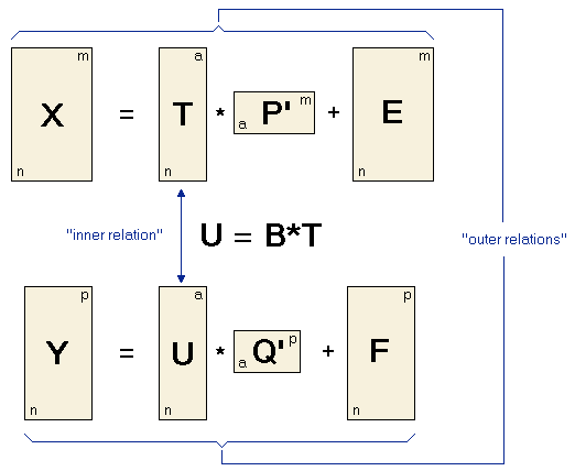
From H. Lohninger http://www.statistics4u.com
Regression beyond ordinary least squares
- Ordinary least-squares inference commonly assumes independent errors with constant variance; normality supports exact small-sample tests.
- Weighted least squares models unequal precision, for example with
lm(..., weights = w). - Generalised linear models specify a response distribution and link, for example
glm(..., family = binomial()). - Robust regression, such as
MASS::rlm(), reduces sensitivity to particular deviations such as outliers.
A GLM does not automatically solve correlated errors.
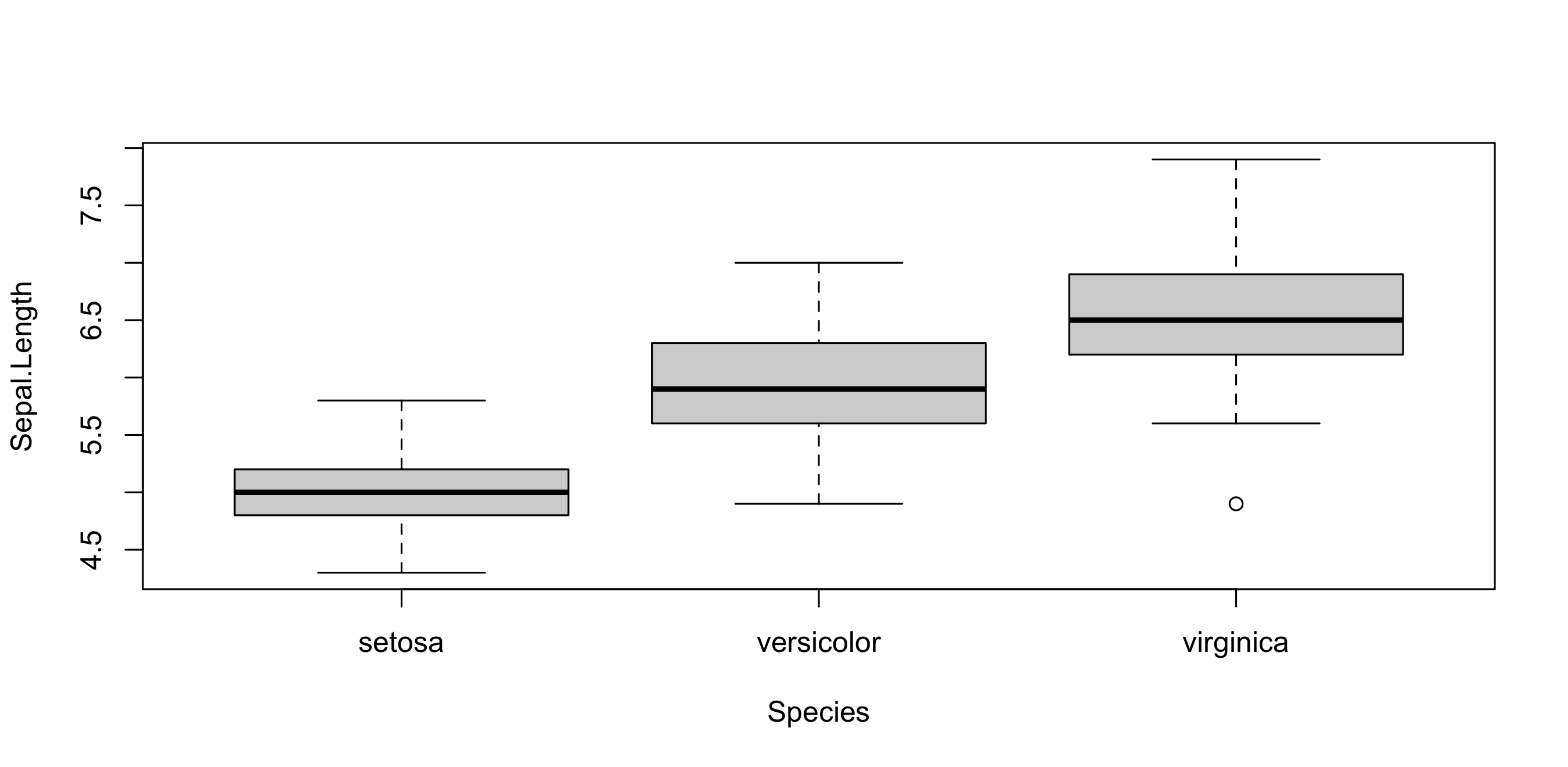
One way anova (1/2)
Generalization of t-test
H_0: \mu_0=\mu_1=\cdots=\mu_p
    One-way analysis of means (not assuming equal variances)

data:  Sepal.Length and Species
F = 138.91, num df = 2.000, denom df = 92.211, p-value < 2.2e-16- p-value small: we reject null hypothesis of equal means
One way anova (2/2)
Anova
Analysis of Variance Table

Model 1: Sepal.Length ~ 1
Model 2: Sepal.Length ~ Species - 1
  Res.Df     RSS Df Sum of Sq      F    Pr(>F)
1    149 102.168
2    147  38.956  2    63.212 119.26 < 2.2e-16 ***
---
Signif. codes: 0 '***' 0.001 '**' 0.01 '*' 0.05 '.' 0.1 ' ' 1Principal Component Analysis: model
Importance of components:
                          PC1    PC2     PC3     PC4
Standard deviation     1.7084 0.9560 0.38309 0.14393
Proportion of Variance 0.7296 0.2285 0.03669 0.00518
Cumulative Proportion 0.7296 0.9581 0.99482 1.00000 PC1 PC2 PC3 PC4
Sepal.Length 0.5210659 -0.37741762 0.7195664 0.2612863
Sepal.Width -0.2693474 -0.92329566 -0.2443818 -0.1235096
Petal.Length 0.5804131 -0.02449161 -0.1421264 -0.8014492
Petal.Width 0.5648565 -0.06694199 -0.6342727 0.5235971Principal Component Analysis: prediction
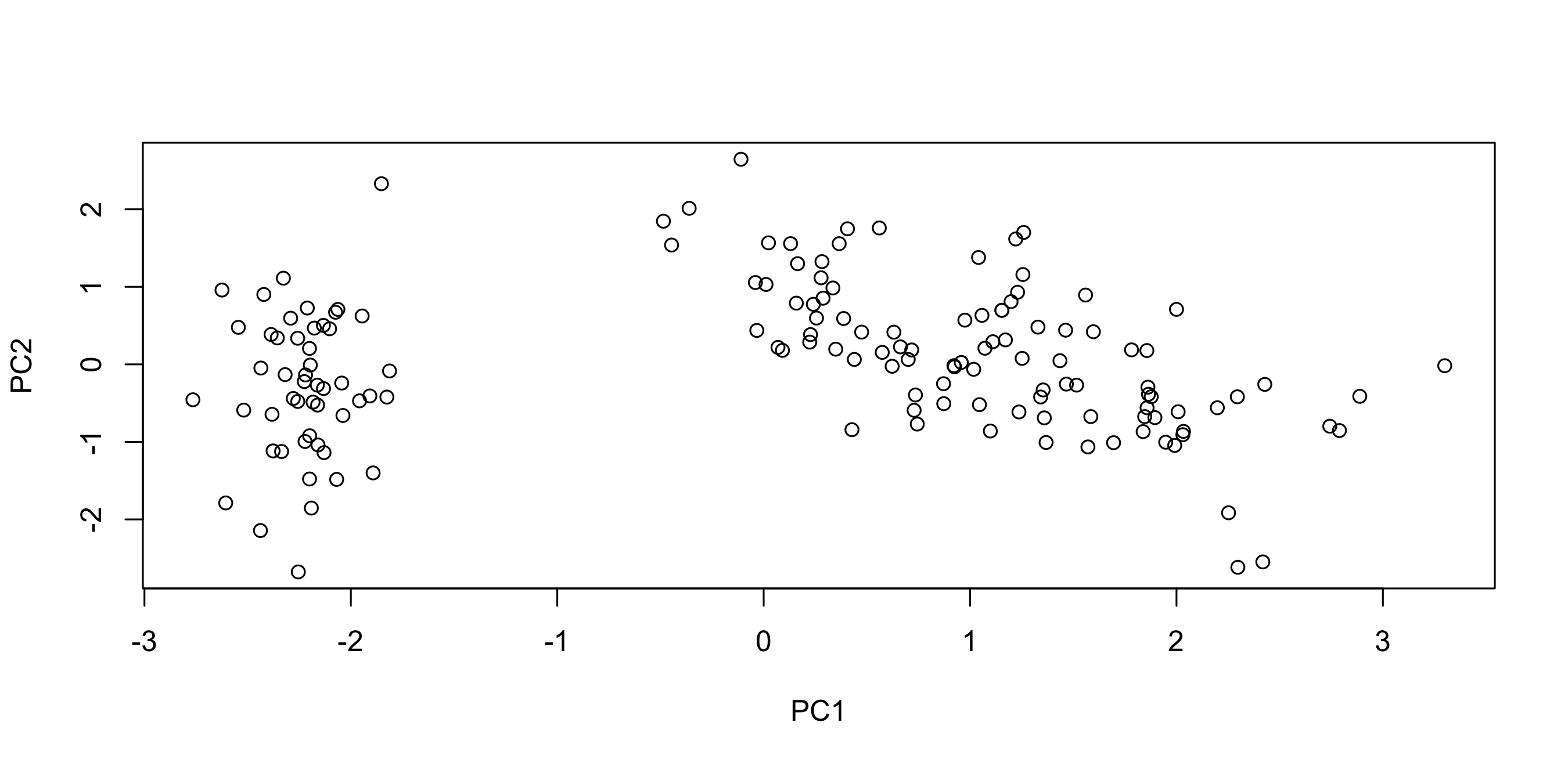
Principal Component Analysis: prediction (1/3)
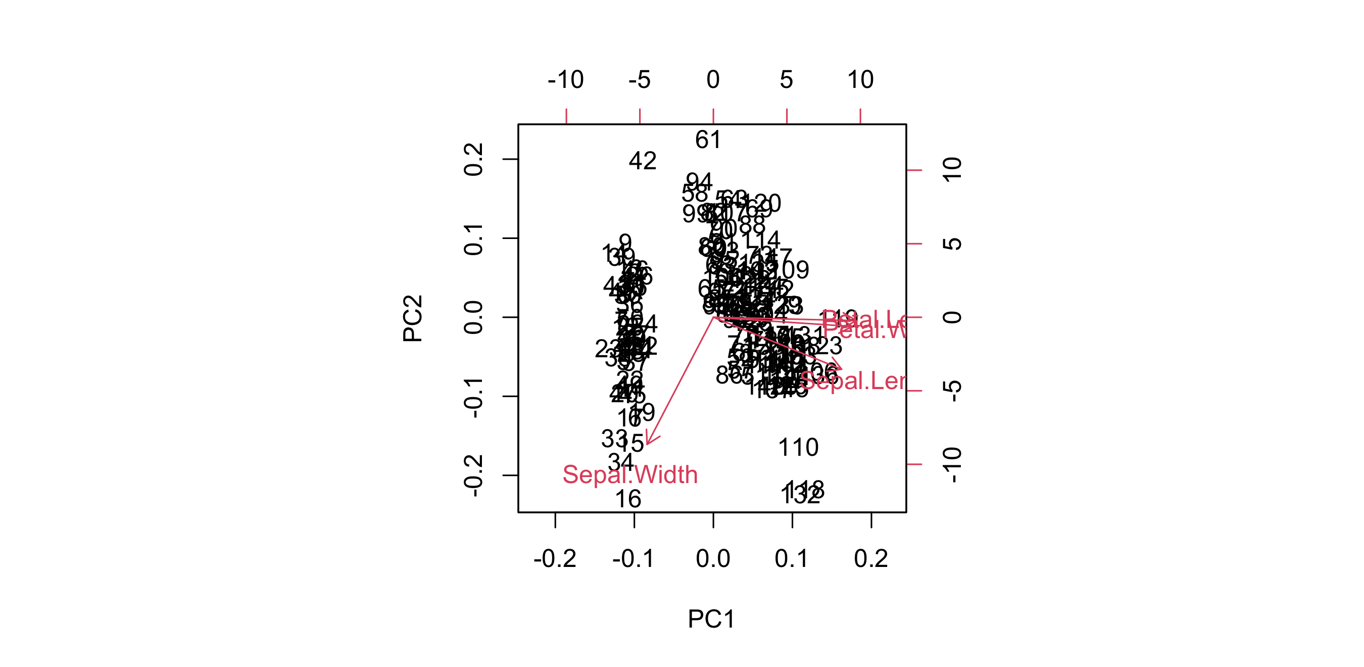
Principal Component Analysis: prediction (2/3)
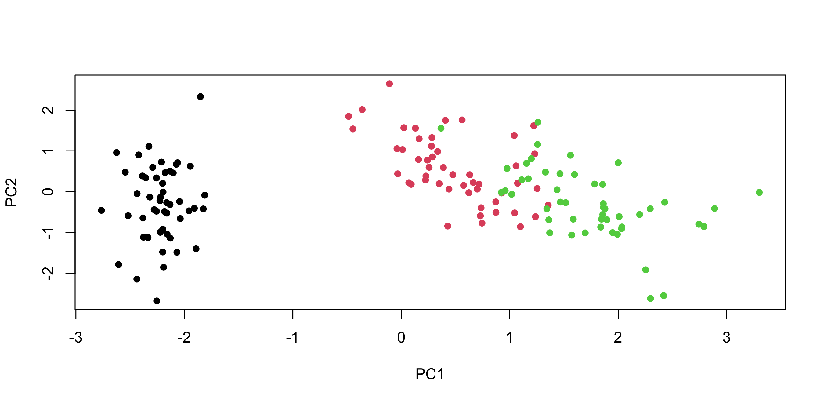
Principal Component Analysis: prediction (3/3)
The End


Bioinformatics · UPC · b2slab